Download

1 / 67
670 likes | 849 Vues
Fault Tolerance in Protein Interaction Networks: Stable Bipartite Subgraphs and Redundant Pathways. Lenore Cowen Tufts University . Protein-protein interaction. Protein-protein interaction. PPI: A simple graph model. vertices ↔ genes/proteins edges ↔ physical interactions.

E N D
Fault Tolerance in Protein Interaction Networks:Stable Bipartite Subgraphs and Redundant Pathways Lenore Cowen Tufts University
PPI: A simple graph model vertices ↔ genes/proteins edges ↔ physical interactions • simplifications: • undirected • loses temporal information • difficult to decompose into separate processes • conflates different PPI types into one class of "physical interactions"
Current data • High-throughput methods are allowing us to fill in many edges in our simple model, often between unannotated proteins.
What we want: What we have: Question: Can we infer anything about "real" pathways from the low-resolution graph model of pairwise interactions?
Interaction types • We distinguish here between two types of interaction: • physical interactions • genetic interactions
Genetic interactions (epistasis) Only 18% of yeast genes are essential (the yeast dies when they’re removed). gene deleted. essential gene. yeast. yeast dies.
Genetic interaction:synthetic lethality Some pairs of nonessential genes exhibit interesting correlative relationships. both genes deleted at once. gene deleted. gene deleted. nonessential gene. nonessential gene. yeast dies. yeast lives.
Nonessential Genes • Some genes are non-essential because they are only required under certain conditions (i.e. an enzyme to metabolize a particular nutrient). • Other genes are non-essential because the network has some built-in redundancy. • One gene (completely or partially) compensates for the loss of another. • One functional pathway (completely or partially) compensates for the loss of another.
In reality, the data are very incomplete:Between-Pathway Model (BPM)
Kelley and Ideker (2005) and Ulitsky and Shamir (2007) • Goal: detect putative BPMs in yeast interactome • Method: • find densely-connected subsets of the physical protein-protein interaction (PI) network (putative pathways) • check the genetic interaction (GI) network to see if patterns in density of genetic interactions correlate with these putative pathways • check resulting structures for overrepresentation of biological function (gene set enrichment)
Kelley and Ideker (2005) and Ulitsky and Shamir (2007) (1) (2) enriched for function X enriched for function Y (3)
Kelley and Ideker (2005) and Ulitsky and Shamir (2007) • Problems: • Sparse data limits the potential scope of discovery • independent validation is difficult
Our method • We show how to systematically search for stable bipartite subgraphs (putative BPMs) • We use only synthetic lethality interactions to search for BPMs: • allows the use of PIs for independent statistical validation of putative BPMs • scope of potential discovery is greater than when using PIs as seed structures
Maximum bipartition • Definition: Given any graph G, a maximum bipartition of G is an assignment of each node of G to one of two sets, A and B, in such a way that the number of edges that CROSS the partition is maximized.
Maximum bipartition Definition: Given any graph G, a maximum bipartition of G is an assignment of each node of G to one of two sets, A and B, in such a way that the number of edges that CROSS the partition is maximized. Fact: Maximum bipartition is NP-hard.
We don’t want a maximum bipartition anyway! We don’t want to force a choice of sides!
Maximal bipartition Definition: Given any graph G, a maximal bipartition of G is an assignment of each node of G to one of two sets, in such a way that moving any single node from one set to the other does not increase the number of edges of G which cross between the two sets.
Algorithm • Randomly assign a set-label to each node in G. • Call a node v “happy” if at least half of its neighbors are in the opposite set from v, and “unhappy” otherwise. • While there exists an unhappy node: • Pick one such node at random. • Flip its set label.
Algorithm (an “unhappy” node flips to “happy.”)
Algorithm Claim: This procedure terminates in at most |E| steps, where |E| is the number of edges in G. Proof: While a particular node may switch its affiliation many times over the course of the algorithm, notice that each time a flip is performed, the number of edges crossing between the two partitions increases by at least one. So there can be at most |E| steps.
Algorithm Claim: On termination, every node is “happy.” Proof: [This is just the termination condition of the while-loop.] Observe that the partition generated in this way is maximal: flipping any single node cannot increase the number of edges crossing between partitions, because all nodes are happy.
Stable Bipartite Subgraph: Motivation If a gene exists within a BPM, then we expect the two pathways of the BPM to fall into opposite sets within most maximal partitions (because the partitioning algorithm is looking to maximize the number of edges crossing between sets). So in a maximal partition, genes in the same pathway as a BPM gene gshould tend to be assigned to the same set as g; those in the opposite pathway should wind up in the opposite set; and those in neither pathway should bounce around with little or no correlation to g’s set-assignment.
Stable Bipartite Subgraph Definition: For a node m, repeat this procedure k times to find maximal bipartite subgraphs. Let A be the set of nodes that occur in the same partition as m at least r percent of the time. Let B be the set of nodes that occur in the opposite partition of m at least r percent of the time. Return A and B as m’s stable bipartite subgraph.
Stable Bipartite Subgraph Definition: For a node m, repeat this procedure k times to find maximal bipartite subgraphs. Let A be the set of nodes that occur in the same partition as m at least r percent of the time. Let B be the set of nodes that occur in the opposite partition of m at least r percent of the time. Return A and B as m’s stable bipartite subgraph. The stable bipartite subgraphs are our BPMs! (k=250; r= 70 percent)
Test Datasets • original physical + genetic interaction data used in Kelley + Ideker (2005) • up-to-date set of physical + genetic interactions taken from BioGRID database (October 2007) 682 genes (nodes) 1,858 edges (SL interactions) 1,678 genes (nodes) 6,818 edges (SL interactions)
How do we know it is meaningful? Biological validation: Enrichment results. We find things that are known to be functionally related in our putative pathways. [GO Enrichment] Statistical validation: - Location of known PI edges - Prediction of new SL edges
Results SGD GO-SLIM coverage
Website http://bcb.cs.tufts.edu/.yeast.bpm/
Website http://bcb.cs.tufts.edu/.yeast.bpm/
Website http://bcb.cs.tufts.edu/.yeast.bpm/
Results: BPM Validation In addition to validation based on coherence of biological function, we can also statisticially validate our methods directly from the structure of the network! Method 1: Examine the distribution of known PIs within each BPM.
Results: BPM Validation Goal: estimate the probability of seeing as many or fewerphysical interactions betweenthe two sets as were actually observed.
Results: BPM Validation Method 2: Examine the distribution of new SL interactions appearing within each BPM in the Kelley/Ideker network.
Results: BPM Validation Goal: estimate the probability of seeing as many or more newsynthetic-lethality interactions appearing betweenthe two sets as were actually observed.
Results: BPM Validation • Results: Across the set of 175 candidate BPMs from G which contained at least 20 new SL edges in G+, the average probability that the observed between-pathway bias would occur by chance was 0.017. • Since these new edges were not used to construct candidate BPMs in G, their distribution bias provides independent support for the hypothesis that stable subgraphs do indeed correspond to biologically meaningful structures.