Download

1 / 16
160 likes | 256 Vues
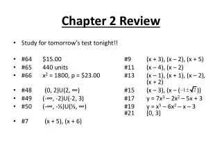
Chapter 2 Review. Group Members: Aditya “ dits ” Shah Alex “ wu -tang” Wu Akash “try-hard” Doshi. The Big Idea.

E N D
Chapter 2 Review Group Members: Aditya “dits” Shah Alex “wu-tang” Wu Akash “try-hard” Doshi
The Big Idea • A variable’s location in a distribution can be described by its standardized form or percentile. Many real life situations, such as grades and population growth, follow a type of distribution called Normal distribution. Finding a variable’s location in this distribution is the most important part of this chapter.
Vocabulary You Need to Know • Density curve • Normal distribution • Normal curve • Z-score • Standardization • Percentile • Normal probability plot
Density Curves • These curves give us a mathematical model for distributions • They are either on or above the horizontal axis and have an area of 1 underneath • For density curves our median is the equal areas point and the mean is the “balance point” • We can tell a curve is skewed if the mean is pulled towards the tail
Normal Distribution • Normal distribution is classified as a continuous, symmetrical, bell-shaped distribution of a variable • Other characteristics are that the mean, median, and mode are all equal and located at the middle of the curve. • The curve is unimodal (one mode) and it never touches the x-axis (the axis acts like an asymptote) • AREA UNDER THE CURVE IS EQUAL TO 1!!
Empirical Rule • The 68-95-99.7 rule • 68% of all data lies within 1 standard dev. from the mean. 95% of all data lies within 2 standard dev. from the mean. 99.7% of all data lies within 3 standard dev. from the mean. • We use empirical rule to predict outcomes, estimate impending data, etc.
Z-Score • Z= • We use z scores to standardize x values • If z is negative, use the table on the left-hand page • If z is positive, use the table on the right-hand page • When working backwards, find the “p” value you are given on the table in your book/given. If we say our p=.95 we look for where a z-score equals this. In this case it is halfway between .9495 and .9505, so we average the z-scores 1.64 and 1.65 to get a final z-score of 1.645.
Normal Probability Plot • This is a graphical technique for normality testing-whether or not a data set is normally distributed • The data are plotted against a theoretical normal distribution in such a way that the points should form an approximate straight line. Deviations from this straight line indicate departures from normality.
Formulas You Should Know • z = • Empirical rule:- Approximately 68% of observations fall within 1σ from the mean - Approximately 95% of observations fall within 2σ from the mean - Approximately 99.7% of observations fall within 3σ from the mean • z-score conversion to proportion/percentile
Calculator Key Strokes • 1st keystroke: - The normal cumulative distribution function - This finds the area under a normal curve up to some standardized point - Press 2nd-> Vars -> normalcdf( - Enter the lower bound, upper bound, mean, and standard deviation in that order (math print will facilitate this lawlz) - Hit enter and see your area • 2nd keystroke: • The inverse normal distribution function • This finds the z-score of some upper bound for a given area • Press 2nd -> Vars -> invnorm • Enter the area under the curve, mean, and standard deviation • Hit enter and see your area
Example Problem(s) • The weights of packages of ground beef are normally distributed d s bued with mean 1 pound and standard deviation .10. What is the probability that a randomly selected package weighs between 0.80 and 0.85 pounds? • A Company produces “20 ounce” bottles of water. The true amounts of water in the bottles of this brand follow a normal distribution. Suppose the companies “20 ounce” bottles follow a normally distribution with a mean μ=20.2 ounces with a standard deviation σ=0.125 ounces. What proportion of the jars are under‐filled (i.e.,have less than 20 ounces of water)? • What proportion of the water bottles contain between 20 and 20.3 ounces of water. • 99% of the bottles of water will contain more than what amount of water?
Helpful Hints • For empirical rule: before applying the rule it’s a good idea to identify the data being described and the mean and standard dev. ALWAYS SKETCH A GRAPH with all the information to help visualize the scenario. CHECK TO MAKE SURE YOU CAN USE THE EMPIRACAL RULE (remember the characteristics!!) • Steps: State the problem, use the table, draw and shade a picture, and unstandardize to obtain your x