Verification of Precipitation Areas Beth Ebert Bureau of Meteorology Research Centre

1. Verification of Precipitation Areas Beth Ebert Bureau of Meteorology Research Centre Melbourne, Australia e.ebert@bom.gov.au

2. Outline 1. “Eyeball” verification - use of maps 2. QPF verification using gridpoint match-ups 3. Space-time verification of pooled data 4. Entity-based (rain “blob”) verification 5. Summary

3. 1. “Eyeball” verification - some examples Accumulated rain over eastern Germany and western Poland, 4-8 July 1997

4. WWRP Sydney 2000 Forecast Demonstration Project

5. RAINVAL - Operational verification of NWP QPFs

6. . . . . . . . . . . . . . . . . Observed Forecast . . . . . . . . . . . . . . . . . . . . . . . . . . . . . . . . . . . . . . . . . . . . . . . . . . . . . . . . . . . . . . . . . . . . . . . . . . . . . . . . . . . . . . . . . . . . . . . . . . . . . . . . . . . . . . . . . . • 2. QPF verification using (grid)point match-ups • All verification statistics can be applied to spatial estimates when treated as a matched set of forecasts/observations at a set of individual points! Method 1: Analyze observations onto a grid

7. Observed Forecast Method 2: Interpolate model forecast to station locations Q: Which verification approach is better? A: It depends!

8. Arguments in favor of grid: • point observations may not represent rain in local area • gridded analysis of observations better represents the grid-scale values that a model predicts • spatially uniform sampling • Use to verify gridded forecasts • Arguments in favor of station locations: • observations are “pure” (not smoothed or interpolated) • Use to verify forecasts at point locations or sets of point locations • Note: Verification scores improve with increasing scale!

9. Preparation of gridded (rain gauge) verification data: • Real time vs. non-real time • Quality control to eliminate bad data • Mapping procedure: • simple gridbox average • objective analysis (Barnes, statistical interpolation, kriging, splines, etc.) • Map observations to model grid • Model intercomparison - map to common grid • Uncertainty in gridbox values

10. Continuous statistics quantify errors in forecast rain amount

11. Categorical statistics quantify errors in forecast rain occurrence

12. Verification of QPFs from NWP models Vary rain threshold from light to heavy Bias score Equitable threat score

13. Verification of NWP QPFs over Germany equitable threat w.r.t. chance equitable threat w.r.t. persistence

14. Verification of nowcasts in Sydney 2000 FDP —— Nowcast - - - - Persistence

15. 3. Space-time QPF verification (a) Pool forecasts and observations in SPACE AND TIME  summary statistics

16. Caution: Results may mask regional and/or seasonal differences summer Model performance in Australian tropics annual winter

17. No data 0.0-0.2 0.2-0.4 0.4-0.6 0.6-0.8 0.8-0.9 0.9-1.0 1.0-1.1 1.1-1.2 1.2-1.5 1.5-2.0 2.0-3.0 3.0-4.0 (b) Pool forecasts and observations in SPACE but NOT TIME  maps of temporal statistics Bias score June 1995-November 1996

18. (c) Pool forecasts and observations in TIME but NOT SPACE  time series of spatial statistics OBS LAPS 24 h LAPS 36 h LAPS 48 h 1-30 Apr 2001 Australian region

19. Limitations toQPF verification using (grid)point match-ups: • Some seemingly good verification statistics may result from compensating errors • too much rain in one part of the domain offset by too little rain in another part of the domain • interseasonal rainfall variation captured but shorter period variation not captured • Conservative forecasts are rewarded • Some rain forecasts look quite good except for the location of the system; unfortunately, traditional verification statistics severely penalize these cases

20. Observed Forecast • 4. Entity-based QPF verification (rain “blobs”) • Verify the properties of the forecast rain system against the properties of the observed rain system: • location • rain area • rain intensity (mean, maximum)

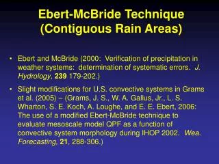
21. Define a rain entity by a Contiguous Rain Area (CRA), a region bounded by a user-specified isohyet. Some possible choices of CRA thresholds are: 1 mm d-1: ~ all rain in system 5 mm d-1: “important” rain 20 mm d-1: rain center Observed Forecast

22. Observed Forecast • Determining the location error: • Horizontally translate the QPF until the total squared error between the forecast and the analysis (observations) is minimized in the shaded region. • The displacement is the vector difference between the original and final locations of the forecast. Arrow shows optimum shift.

23. CRA error decomposition The total mean squared error (MSE) can be written as: MSEtotal = MSEdisplacement + MSEvolume+ MSEpattern The difference between the mean square error before and after translation is the contribution to total error due to displacement, MSEdisplacement = MSEtotal – MSEshifted The error component due to volume represents the bias in mean intensity, where and are the CRA mean forecast and observed values after the shift. The pattern error accounts for differences in the fine structure of the forecast and observed fields, MSEpattern = MSEshifted - MSEvolume

24. Example: Nowcasts from Sydney 2000 FDP

25. Example: Australian regional NWP model

26. Rain area Mean rain intensity North of 25°S South of 25°S

27. Rain volume Maximum rain intensity

28. Displacement error

29. Event forecast classification • Two most important aspects of a “useful” QPF: • Location of predicted rain must be close to the observed location • Predicted maximum rain rate must be “in the ballpark”

30. Example: Proposed event forecast criteria for 24h NWP QPFs Good location: Forecast rain system must be within 2° lat/lon or one effective radius of the rain system, but not farther than 5° from the observed location Good intensity: Maximum rain rate must be within one category of observed (using rain categories of 1-2, 2-5, 5-10, 10-25, 25-50, 50-100, 100-150, 150-200, >200 mm d-1) Event forecast classification Australian 24h QPFs from BoM regional model, July 1995-June 1999 (2066 events)

31. Error decomposition Australian 24h QPFs from BoM regional model, July 1995-June 1999 (2066 events)

32. Advantages of entity-based QPF verification: • intuitive, quantifies “eyeball” verification • addresses location errors • allows decomposition of total error into contributions from location, volume, and pattern errors • rain event forecasts can be classified as "hits", "misses", etc. • does not reward conservative forecasts • Disadvantages of entity-based verification: • more than one way to do pattern matching (i.e., not 100% objective • forecast must resemble observations sufficiently to enable pattern matching

33. Precision Objective (grid)point match-ups entities Meaning Subjective maps Point Area 5. Summary Spatial QPF success* can be qualitatively and quantitatively measured in many ways, each of which tells only part of the story *Note: “success” depends on the requirements of the user!!