Download
1 / 20
200 likes | 207 Vues
Lec 7. Higher Order Systems, Stability, and Routh Stability Criteria. Higher order systems Stability Routh Stability Criterion Reading: 5-4; 5-5, 5.6 (skip the state-space part). TexPoint fonts used in EMF. Read the TexPoint manual before you delete this box.: A A A A.

E N D
Lec 7. Higher Order Systems, Stability,and Routh Stability Criteria • Higher order systems • Stability • Routh Stability Criterion • Reading: 5-4; 5-5, 5.6 (skip the state-space part) TexPoint fonts used in EMF. Read the TexPoint manual before you delete this box.: AAAA
Nonstandard 2nd Order Systems So far we have been focused on standard 2nd order systems Non-unit DC gain: Extra zero:
Effect of Extra Zero standard form Under any input, say, unit step signal, the response of H(s) is unit-step response of standard 2nd order system
Unit-Step Response (=0.4,=1,n=1) The introduction of the extra zero affects overshoot in the step response.
Higher Order Systems n-th order system: It has n poles p1,…,pn and m zeros z1,…,zm Factored form: As in second order systems, locations of poles have important implications on system responses
Distinct Real Poles Case Suppose the n poles p1,…,pn are real and distinct Partial fraction decomposition of H(s): (parallel connection of n first order systems) where 1,…,n are residues of the poles Impulse response: Step response: The transient terms will eventually vanish if and only if all the poles p1,…,pn are negative (on the LHP)
Distinct Poles (may be complex) Suppose that the n poles p1,…,pn are distinct (may be complex) Partial fraction decomposition of H(s): (parallel connection of qfirst order systems and runderdamped second order systems) The transient terms will eventually vanish if and only if all the poles p1,…,pn have negative real part (on the LHP)
Remarks • Effect of poles on transient response • Each real pole p contributes an exponential term • Each complex pair of poles contributes a modulated oscillation • The magnitude of contribution depends on residues, hence on zeros • Stability of system responses • The transient term will converge to zero only if all poles are on the LHP • The further to the left on the LHP for the poles, the faster the convergence • Dominant poles • Poles with dominant effect on transient response • Can be real, or complex conjugate pair
Stability of Systems • One of the most important problems in control (ex. aircraft altitude control, driving cars, inverted pendulum, etc.) • System is stable if, under bounded input, its output will converge to a finite value, i.e., transient terms will eventually vanish. Otherwise, it is unstable • A system modeled by a transfer function is stable if all poles are on the open left half of the complex plane
Problems Related to Stability Stability Criterion: for a given system, determine if it is stable controller plant + Stabilization: for a given system that may be unstable, design a feedback controller so that the overall system is stable.
How to Determine Stability Transfer function is stable are on the LHP All roots of “stable polynomial” Method 1: Direct factorization Method 2: Routh’s Stability Criterion Determine the # of roots on the LHP, on the RHP, and on j axis without having to solve the equation. • Advantage: • Less computation • Works when some of the coefficients depend on parameters
A Necessary Condition for Stability is stable (assume a00) If Then have the same sign, and are nonzero Example:
Routh’s Stability Criterion Step 1: determine if all the coefficients of have the same sign and are nonzero. If not, system is unstable Step 2: arrange all the coefficients in the follow format “Routh array”
Routh’s Stability Criterion (cont.) Step 3: # of RHP roots is equal to # of sign changes in the first column Hence the polynomial is stable if the first column does not change sign Routh array
Example Determine the stability of Check by Matlab command: roots([1 2 3 4 5])
+ Stability vs. Parameter Range Determine the range of parameter K so that the closed loop system is stable Closed loop transfer function Stability of depends on K
Special Case I The first term in one row of the Routh array may become zero Example: Replace the leading zero by Continue to fill out the array and let N+ be the # of sign changes in the first column Let and let N- be the # of sign changes in the first column Let For this example:
Special Case II An entire row of the Routh array may become zero Example: Auxiliary polynomial Derivative of auxiliary polynomial: Roots of auxiliary polynomial are roots of the original polynomial No sign changes in the first column, hence no additional RHP roots See textbook pp. 279 for a more complicated example.