Download
1 / 129
1.29k likes | 1.6k Vues
NUS Turbulence Workshop, Aug. ‘04. Large Eddy Simulation in Aid of RANS Modelling. M A Leschziner Imperial College London. RANS/LES simulation of flow around a highly-swept wing. Collaborators. Lionel Temmerman Anne Dejoan Sylvain Lardeau Chen Wang Ning Li Fabrizio Tessicini

E N D
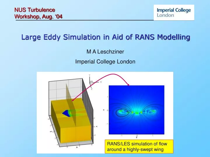
NUS Turbulence Workshop, Aug. ‘04 Large Eddy Simulation in Aid of RANS Modelling M A Leschziner Imperial College London RANS/LES simulation of flow around a highly-swept wing
Collaborators Lionel Temmerman Anne Dejoan Sylvain Lardeau Chen Wang Ning Li Fabrizio Tessicini Yong-Jun Jang Ken-ichi Abe Kemo Hanjalic
The Case for RANS • RANS may be something of a ‘can of worms’, but is here to stay • Decisive advantages: • Economy, especially in • statistical homogeneous 2d flows • when turbulence is dominated by small, less energetic scales • in the absence of periodic instabilities • Good performance in thin shear and mildly-separated flows, especially near walls • Predictive capabilities depend greatly on • appropriateness of closure type and details relative to flow characteristics • quality of boundary conditions • user competence
Challenges to RANS • Dynamics of large-scale unsteadiness and associated non-locality • Massive separation – large energetic vortices • Unsteady separation from curved surfaces • Reattachment (always highly unsteady) • Unsteady instabilities and interaction with turbulence • Strong non-equilibrium conditions • Interaction between disparate flow regions • post reattachment recovery • wall-shear / free-shear layers • Highly 3d straining – skewing, strong streamwise vorticity
Separation from Curved Surfaces - Tall Order for RANS? LES instantaneous realisations Reverse flow RANS
Dynamics of Separated Flow Steady Unsteady Separation
Dynamics of Separated Flow Steady Reattachment Attached Recovery
RANS Developments • Desire to extent generality drives RANS research • Non-linear eddy-viscosity models • Explicit algebraic Reynolds-stress models • Full second-moment closure • Structure-tensor models • multi-scale models… • Simulation plays important role in aiding development and validation • Traditionally, DNS for homogeneous and channel flow at low Re used • Increasingly, LES exploited for complex flow
The Argument for Resolving Anisotropy • Generalised eddy-viscosity hypothesis: • Wrongly implies that eigenvalues of stress and strain tensors aligned • Wrong even in thin-shear flow: Channel flow Which is wrong
The Argument for Resolving Anisotropy • Exact equations imply complex stress-strain linkage • Analogous linkage between scalar fluxes and production • Can be used to demonstrate • Origin of anisotropy in shear and normal straining • Experimentally observed high sensitivity of turbulence to curvature, rotation, swirl, buoyancy and and body forces • Low generation of turbulence in normal straining • Inapplicability of Fourier-Fick law for scalar/heat transport • Inertial damping of near-wall turbulence by wall blocking
Reynolds-Stress-Transport Modelling • Closure of exact stress-transport equations • Modern closure aims at realisability, 2-component limit, coping with strong inhomogeneity and compressibility • Additional equations for dissipation tensor • At least 7 equations in 3D • Numerically difficult in complex geometries and flow • Can be costly • Motivated algebraic simplifications
Homogeneous Straining • Axisymmetric expansion
Homogeneous Straining • Homogeneous shear and plain strain
Near-Wall Shear • Channel flow
Explicit Algebraic Reynolds-Stress Modelling • Arise from the explicit inversion of • Transport of anisotropy (and shear stress) ignored • Redistribution model linear in stress tensor • Lead to algebraic equations of the form • Most recent variant: Wallin & Johansson (2000) • Recent modification (Wallin & Johansson (2002/3)): approximation of anisotropy transport by reference to streamline-oriented frame of reference 0
Non-linear EVM • Constitutive equation • Transport equation for turbulence energy and length-scale surrogate (ε, ω…) • Coefficients determined by calibration Quadratic Quasi-cubic Cubic (=0 in 2d)
Large Eddy Simulation – An alternative? • Superior in wall-remote regions • Resolution requirements rise only with • Near wall, resolution requirement rise with • Near-wall resolution can have strong effect on separation process • Sensitivity to subgrid-scale modelling • At high Re, increasing reliance on approximate near-wall treatments • Wall functions • Hybrid RANS-LES strategies • DES • Immersed boundary method • Zonal schemes • Spectral content of inlet conditions Achilles heal of LES
Realism of LES – Channel Constriction • Effects of Resolution – no-slip condition x=2h x=6h Re=21900 Distance of nodes closest to wall
Sensitivity of Reattachment to Separation Δxreat=7 Δxsep 0.4 0.05
Realism of LES – Channel Constriction • Effects of near-wall treatment (WFs) on 0.6M mesh
Realism of LES – Channel Constriction • Sensitivity to SGS modelling
Realism of LES – Stalled Aerofoil • High-lift aerofoil – an illustration of the resolution problem Re=2.2M Experiments
Realism of LES – Stalled Aerofoil • High-lift aerofoil
Realism of LES – Stalled Aerofoil • Effect of the spanwise extent
Realism of LES – Stalled Aerofoil • Mesh 1: 320 x 64 x 32 = 6.6 • 105 cells • Mesh 2: 768 x 128 x 64 = 6.3 • 106 cells • Mesh 3: 640 x 96 x 64 = 3.9 • 106 cells • Mesh 4: 1280 x 96 x 64 = 7.8 • 106 cells • Effect of the mesh Streamwise velocity at x/c = 0.96 Prediction of the friction coefficient
High-Lift Aerofoil - RSTM & NLEVM RSTM NLEVM
The Case for LES for RANS Studies • Experiments traditionally used for validation • Very limited data resolution • Boundary conditions often difficult to extract • Errors – eg 3d contamination in ‘2d’ flow • Reliance on wind-tunnel corrections • Example: 3d hill flow (Simpson and Longe, 2003)
New Experimental Information • Flow visualisation vs. LDV x/H 0.18 separation in oilflow x/H 0.7 attachment in oilflow x/H 2.0 attachment in oilflow Large bump#3 Separation in CCLDV data x/H 1.5 separation in oilflow
The Case for LES for RANS Studies • Well-resolved LES a superior alternative • Close control on periodicity and homogeneity • Reliable assessment of accuracy • SGS viscosity and stresses relative to resolved • Spectra and correlations • Ratio of Kolmogorov to grid scales • Balance of budgets (eg zero pressure-strain in k-eq.) • Reliable extraction of boundary conditions • Second and possibly third moments available • Budgets available • Attention to resolution and detail essential
LES for RANS Studies • Considered are five LES studies contributing to RANS • 2d separation from curved surfaces • 3d separation from curved surfaces • Wall-jet • Separation control with periodic perturbations • Bypass transition
Study of Non-Linear EVMs for Separation Constitutive equation Quadratic Quasi-cubic Cubic (=0 in 2d)
2C-Limit Non-linear EVM • Recent forms aim to adhere to wall-asymptotic behaviour • Example: NLEVM/EASM of Abe, Jang & Leschziner (2002) • Anisotropy cannot be represented by functions of alone • Thus, addition of near-wall-anisotropy term, calibrated by reference to channel-flow DNS • Involve “wall-direction indicators”, , Kolmogorov as well as macro time scales and viscous-damping function ld
2C-Limit Non-Linear EVM • Performance of AJL model in channel flow ( and variants) by reference to DNS
2C-Limit Non-linear EVM Performance of AJL model in channel flow ( and variants) Turbulence energy budget
A-priori Study of Non-Linear EVMs • Quadratic terms represent anisotropy • ‘cubic’ terms represent curvature effects • Example: • Streamwise normal stress across separated zone • Accurate simulation data used for model investigation • Modelled stresses determined from constitutive equation with mean-flow solution inserted • Comparison with simulated stresses • Linear, quadratic and cubic contributions can be examined separately 2d periodic hill, Re=21500 Jang et al, FTC, 2002
Highly-Resoved LES Data • Two independent simulations of 5M mesh
Highly-Resolved LES Data Near-wall velocity profiles at 3 streamwise locations (wall units) Turbulence-energy budget at x/h = 2.0 IJHFF (2003), JFM (2005)
Highly-Resolved LES Data - Animations U-velocity W-velocity Q-criterion Pressure
Streamlines LES k- Abe et al
A-priori Study – modelled vs. simulated stresses Linear EVM uv uu Quadratic 2c limit EVMAbe,Jang &Leschziner, 2003 uu (quadr) uu (linear)
A-priori Study – modelled vs. simulated stresses Linear EVM uu uv Cubic EVMCraft, Launder & Suga, 2003 uu (linear) uu (‘cubic’) uu (quadr)
A-priori Study – modelled vs. simulated stresses Linear EVM uu uv Explicit ASM Wallin &Johansson, 2000 uu (linear) uu (quadr.)
3D-Hill - Motivation Efforts to predict flow around 3d hill with anisotropy-resolving closures LDA Experiments by Simpson et al (2002) Re=130,000, boundary-layer thickness = 0.5xh Computations with up to 170x135x140 (=3.3 M) nodes Several NLEVMs and RSTMs
Topology – Experiment vs. NLEVM Computation Chen et al, IJHFF, 2004
3D Hill - LES • Can origin of discrepancies be understood? • Wall-resolved LES at Re=130,000 deemed too costly • LES and RSTM computations undertaken at Re=13,000 • Identical inlet conditions as at Re=130,000 • Grid: 192 x 96 x 192 = 3.5M cells (y+=O(1)) • LES scheme • Second-order + ‘wiggle-detection’, fractional-step, Adams- Bashforth • Solves pressure equation with SLOR + MG • Fully parallelised • WF and LES/RANS hybrid near-wall approximations • SGS models: Smag + damping, WALE Temmerman et al, ECCOMAS, 2004
Computational Aspects - LES Re=13000 128 x 64 x 128 cells CFL=0.2 d=0.003 CPU cost: 32 x 30 CPUh on Itanium2 cluster Statistics connected over 10 flow-through times, after initial 6 initial sweeps Near-wall grid: