FPGA vs. GPU for Sparse Matrix Vector Multiply

1. FPGA vs. GPU forSparse Matrix Vector Multiply Yan Zhang, Yasser H. Shalabi, Rishabh Jain, Krishna K. Nagar, Jason D. Bakos Dept. of Computer Science and Engineering University of South Carolina Heterogeneous and Reconfigurable Computing Group http://herc.cse.sc.edu This material is based upon work supported by the National Science Foundation under Grant Nos. CCF-0844951 and CCF-0915608

2. Sparse Matrix Vector Multiplication • SpMV used as a kernel in many methods • Iterative Principal Component Analysis (PCA) • Matrix Decomposition: LU, SVD, Cholesky, QR, etc • Iterative Linear System Solvers: CG, BCG, GMRES, Jacobi etc • Other Matrix Operations

3. Talk Outline • GPU • Microarchitecture & Memory Hierarchy • Sparse Matrix Vector Multiplication on GPU • Sparse Matrix Vector Multiplication on FPGA • Analysis of FPGA and GPU Implementations

4. NVIDIA GT200 Microarchitecture • Many-core architecture • 24 or 30 On-chip Streaming Multiprocessors • 8 Scalar Processor per SMs • Each SP can issue up to four threads • Warp: Group of 32 threads having common control path

5. GPU Memory Hierarchy Multiprocessor 1 Multiprocessor n Multiprocessor 2 • Off-Chip Device Memory • On board • Host and GPU exchange I/O data • GPU stores state data • On-Chip Memories • A large Set of 32-bit regs per processor • Shared Memory • Constant Cache (Read Only) • Texture Cache (Read Only) Texture Memory Constant Memory Texture Constant Device Memory

6. GPU Utilization and Throughput Metrics • CUDA Profiler used to measure • Occupancy • Ratio of active warps to the maximum number of active warps per SM • Limiting Factors: • Number of registers • Amount of shared memory • Instruction count required by the threads • Not an accurate indicator of SM utilization • Instruction Throughput • Ratio of achieved instruction rate to peak instruction rate • Limiting Factors: • Memory latency • Bank conflicts on shared memory • Inactive threads within a warp caused by thread divergence

7. Talk Outline • GPU • Memory Hierarchy & Microarchitecture • Sparse Matrix Vector Multiplication on GPU • Sparse Matrix Vector Multiplication on FPGA • Analysis of FPGA and GPU Implementations

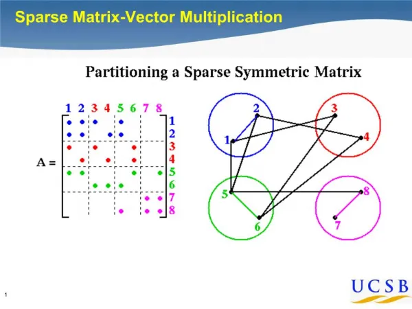
8. Sparse Matrix • Sparse Matrices can be very large but contain few non-zero elements • SpMV: Ax = b • Need special storage format • Compressed Storage Row (CSR)

9. GPU SpMV Multiplication • State of the art • NVIDIA Research (Nathan Bell) • Ohio State University and IBM (Rajesh Bordawekar) • Built on top of NVIDIA’s SpMV CSR kernel • Memory management optimizations added • In general, performance depends on effective use of GPU memories

10. OSU/IBM SpMV • Matrix stored in device memory • Zero padding: Elements per row to be a multiple of sixteen • Input vector in SM’s texture cache • Shared memory stores output vector • Extracting Global Memory Bandwidth • Instruction and variable alignment necessary • Fulfilled by built-in types • Global memory access by all threads of a half-warp coalesced into a transaction of 32, 64, or 128 bytes

11. Analysis • Each thread reads 1/16th of non-zero elements in a row • Accessing device memory (128 byte interface): • Access valarray => 16 threads read 16 x 8 bytes = 128 bytes • Access col array => 16 threads read 16 x 4 bytes = 64 bytes • Occupancy achieved by all matrices was ONE • Each thread uses sufficiently small amount of registers and shared memory • Each SM capable of executing the maximum number of threads possible • Instruction throughput ratio : 0.799 to 0.886

12. Talk Outline • GPU • Memory Hierarchy & Microarchitecture • Sparse Matrix Vector Multiplication on GPU • Sparse Matrix Vector Multiplication on FPGA • Analysis of FPGA and GPU Implementations

13. SpMV FPGA Implementation • Generally Implemented Architecture (from literature) • Multipliers followed by a binary tree of addersfollowed by accumulator • Values delivered serially to the accumulator • For a set of n values, n-1 additions required to reduce • Problem • Accumulation of FP values is an iterative procedure M1 V1 Accumulator M2 V2

14. The Reduction Problem Feedback Loop Basic Accumulator Architecture + Adder Pipeline Partial sums Reduction Ckt Control Required Design Mem Mem

15. Previous Reduction Ckt Implementations • We need better architecture • Feedback Reduction Circuit • Simple and Resource Efficient • Reduce the performance gap between adder and accumulator • Move logic outside the feedback loop

16. A Close Look at Floating Point Addition IEEE 754 adder pipeline (assume 4-bit significand): Compare exponents De-normalize smaller value Add mantissas Round Re-normalize Round 1.1011 x 223 1.1110 x 221 1.1011 x 223 0.01111 x 223 10.00101 x 223 10.0011 x 223 1.00011 x 224 1.0010 x 224

17. Base Conversion • Idea: • Shift both inputs to the left by amount specified in low-order bits of exponents • Reduces size of exponent, requires wider adder • Example: • Base-8 conversion: • 1.01011101, exp=10110 (1.36328125 x 222 => ~5.7 million) • Shift to the left by 6 bits… • 1010111.01, exp=10 (87.25 x 28*2 = > ~5.7 million)

18. Accumulator Design stage 1 stage 2 stages 3 to (3+a-1) stage 3+a stage 4+a stage 5+a stage 6+a stage 7+a base conversion input denormalize 2s complement base+54 + output 64 base+54 renormalize/ base conversion 2s complement denormalize base+54 reassembly sign count leading zeros 64 shift exponenthigh compare /subtract 11-lg(base) 11-lg(base) sign Preprocess Post-process Feedback Loop α= 3

19. Reduction Circuit • Designed a novel reduction circuit • Lightweight by taking advantage of shallow adder pipeline • Requires • One input buffer • One output buffer • Eight State FSM controller

20. Three-Stage Reduction Architecture Input Output buffer “Adder” pipeline Input buffer

21. Three-Stage Reduction Architecture Input Output buffer “Adder” pipeline B1 a3 a2 a1 0 Input buffer

22. Three-Stage Reduction Architecture Input Output buffer “Adder” pipeline B2 B1 a3 a2 a1 Input buffer

23. Three-Stage Reduction Architecture Input Output buffer “Adder” pipeline B3 a1+a2 B1 a3 Input buffer B2

24. Three-Stage Reduction Architecture Input Output buffer “Adder” pipeline B4 B2+B3 a1+a2 B1 a3 Input buffer

25. Three-Stage Reduction Architecture Input Output buffer “Adder” pipeline B5 B1+B4 B2+B3 a1+a2 a3 Input buffer

26. Three-Stage Reduction Architecture Input Output buffer “Adder” pipeline B6 a1+a2+a3 B1+B4 B2+B3 Input buffer B5

27. Three-Stage Reduction Architecture Input Output buffer “Adder” pipeline B7 B2+B3+B6 a1+a2+a3 B1+B4 Input buffer B5

28. Three-Stage Reduction Architecture Input Output buffer “Adder” pipeline B8 B1+B4+B7 B2+B3+B6 a1+a2+a3 Input buffer B5

29. Three-Stage Reduction Architecture Input Output buffer “Adder” pipeline C1 B1+B4+B7 B2+B3+B6 B5+B8 0 Input buffer

30. Reduction Circuit Configurations • Four “configurations”: • Deterministic control sequence, triggered by set change: • D, A, C, B, A, B, B, C, B/D • Minimum set size: α ⌈ lgα + 1⌉-1 • Minimum set size for adder pipeline depth of 3 is 8

31. New SpMV Architecture • Built on top of limitation of Reduction Circuit • Delete Adder Binary tree • Replicate accumulators • Schedule data to process multiple dot products in parallel

32. Talk Outline • GPU • Memory Hierarchy & Microarchitecture • Sparse Matrix Vector Multiplication on GPU • Sparse Matrix Vector Multiplication on FPGA • Analysis of FPGA and GPU Implementations

33. Performance Figures

34. Performance Comparison If FPGA Memory bandwidth scaled by adding multipliers/ accumulators to match GPU Memory Bandwidth for each matrix separately

35. Conclusions • Presented state of the art GPU Implementation of SpMV • Presented a new SpMV Architecture for FPGA • Based on novel Accumulator architecture • GPUs at present, perform better than FPGAs for SpMV • Due to available memory bandwidth • FPGAs have the potential to outperform GPUs • Need more memory bandwidth

36. Acknowledgement • Dr. Jason Bakos • Yan Zhang, Tiffany Mintz, Zheming Jin, Yasser Shalabi, Rishabh Jain • National Science Foundation Questions?? Thank You!!

37. Performance Analysis • Xilinx Virtex-2Pro100 • Includes everything related to the accumulator (LUT based adder)