Download
1 / 96
980 likes | 1.52k Vues
Satisfying Assumptions of Linear Regression. Correcting violations of assumptions Detecting outliers Transforming variables Sample problem Solving problems with the script Other features of the script Logic for homework problems. Consequences of failing to satisfy assumptions.

E N D
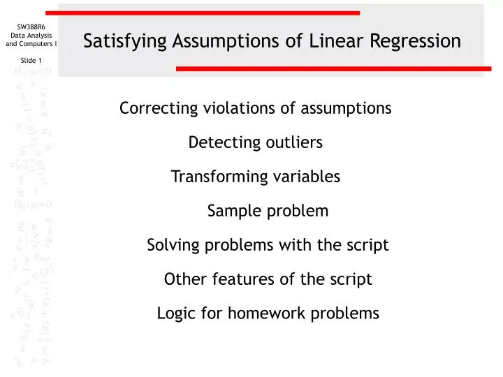
Satisfying Assumptions of Linear Regression • Correcting violations of assumptions • Detecting outliers • Transforming variables • Sample problem • Solving problems with the script • Other features of the script • Logic for homework problems
Consequences of failing to satisfy assumptions • When a regression fails to meet the assumptions, the probabilities that we base our findings on lose their accuracy. Generally, we fail to detect relationships for which we might otherwise have found support, increasing our chances of making a type II error. • If we are using the regression to model expected values for the dependent variable, our predictions may be biased in that we are systematically making non-random errors for subsets of our population.
Correcting violations of assumptions - 1 • There are three strategies available to us to correct our violations of assumptions: • 1. we can exclude outliers from our analysis • 2. we can transform our variables • 3. we can add a polynomial term (square, cube, etc.) for an independent variable. • Employing one strategy generally has an impact on other the other strategies. For example, transforming a variable may change a case’s status as an outlier. Excluding an outlier reduces the skew of the distribution, thereby improving normality.
Correcting violations of assumptions - 2 • The availability of multiple strategies creates the opportunity to report our findings for a relationship in different ways, requiring us to choose to report one that we can defend. • Unless we test all possible combinations, we cannot be certain that we are reporting the optimal relationship. • When we utilize these remedies, we are required to report them with our findings.
Outliers • Outliers are cases that have data values that are very different from the data values for the majority of cases in the data set. • Outliers are important because they can change the results of our data analysis. • Whether we include or exclude outliers from a data analysis depends on the reason why the case is an outlier and the purpose of the analysis.
Different types of outliers • A case can be an outlier because it has an unusual value for the dependent variable, the independent variable, or both. • A case is an outlier on the dependent variable if it has a very large studentized residual. • A case is an outlier on the independent variable if it has high leverage. • A case is an outlier on both if it has a large value for Cook’s distance.
Detecting outliers • If the absolute value of the studentized residuals is larger than 2.0, it is an outlier. • A leverage value identifies an outlier if it is greater than 2 x (number of IV’s + 1) / number of cases: • A Cook’s distance is an outlier if it is greater than 4 / (number of cases – number of Iv’s – 1) • If a case has outlier values greater than twice the values listed above, we will identify it as an extreme outlier.
Removing outliers • In our problems, we will remove a case from the analysis if it exceeds two or more of the criteria for extreme outliers. • When one extreme outlier is removed, the resulting analysis may reveal one or more additional extreme outliers, which could be subsequently be removed until the resulting analysis does not indicate the presence of any additional extreme outliers. • In our problems, we will only remove extreme outliers once. This allows us to identify a more accurate model that accommodates unusual cases.
Detecting an removing outliers in SPSS • The SPSS regression command allows us to save studentized residuals, Cook’s distances, and leverage values to the data editor. • To remove them from the analysis, we use the Select Cases command. Since we select cases to be included in the analysis, we should write the command to identify cases that are not outliers.
Transformations • Transformations change the shape of a distribution, generally by reducing the skewness to more closely approximate a normal distribution. • We are accustomed to expecting numbers on a decimal scale, but mathematically there are may scales for number, e.g. binary, octal, hexadecimal, as well as geometric scales. • Transformations are legitimate as long as they preserve the numeric properties of the numbers.
Transformations change the measurement scale In the diagram to the right, the values of 5 through 20 are plotted on the different scales used in the transformations. These scales would be used in plotting the horizontal axis of the histogram depicting the distribution. When comparing values measured on the decimal scale to which we are accustomed, we see that each transformation changes the distance between the benchmark measurements. All of the transformations increase the distance between small values and decrease the distance between large values. This has the effect of moving the positively skewed values to the left, reducing the effect of the skewing and producing a distribution that more closely resembles a normal distribution.
Transformations:Computing transformations in SPSS • In SPSS, transformations are obtained by computing a new variable. SPSS functions are available for the logarithmic (LG10) and square root (SQRT) transformations. The inverse transformation uses a formula which divides minus one by the original value for each case. • For each of these calculations, there may be data values which are not mathematically permissible. For example, the log of zero is not defined mathematically, division by zero is not permitted, and the square root of a negative number results in an “imaginary” value. We will adjust the values passed to the function to make certain that these illegal operations do not occur.
Transformations:Two forms for computing transformations • There are two forms for each of the transformations to induce normality, depending on whether the distribution is skewed negatively to the left or skewed positively to the right. • Both forms use the same SPSS functions and formula to calculate the transformations. • The two forms differ in the value or argument passed to the functions and formula. The argument to the functions is an adjustment to the original value of the variable to make certain that all of the calculations are mathematically correct.
Transformations:Functions and formulas for transformations • Symbolically, if we let x stand for the argument passes to the function or formula, the calculations for the transformations are: • Logarithmic transformation: compute log = LG10(x) • Square root transformation: compute sqrt = SQRT(x) • Inverse transformation: compute inv = -1 / (x) • Square transformation: compute s2 = x * x • For all transformations, the argument must be greater than zero to guarantee that the calculations are mathematically legitimate.
Transformations:Transformation of positively skewed variables • For positively skewed variables, the argument is an adjustment to the original value based on the minimum value for the variable. • If the minimum value for a variable is zero, the adjustment requires that we add one to each value, e.g. x + 1. • If the minimum value for a variable is a negative number (e.g., –6), the adjustment requires that we add the absolute value of the minimum value (e.g. 6) plus one (e.g. x + 6 + 1, which equals x +7).
Transformations:Example of positively skewed variable • Suppose our dataset contains the number of books read (books) for 5 subjects: 1, 3, 0, 5, and 2, and the distribution is positively skewed. • The minimum value for the variable books is 0. The adjustment for each case is books + 1. • The transformations would be calculated as follows: • Compute logBooks = LG10(books + 1) • Compute sqrBooks = SQRT(books + 1) • Compute invBooks = -1 / (books + 1)
Transformations:Transformation of negatively skewed variables • If the distribution of a variable is negatively skewed, the adjustment of the values reverses, or reflects, the distribution so that it becomes positively skewed. The transformations are then computed on the values in the positively skewed distribution. • Reflection is computed by subtracting all of the values for a variable from one plus the absolute value of maximum value for the variable. This results in a positively skewed distribution with all values larger than zero.
Transformations:Transformation of negatively skewed variables • When an analysis uses a transformation involving reflection, we must remember that this will reverse the direction of all of the relationships in which the variable is involved. • Our interpretation of relationships must be reversed if reflection has been used, or we can apply a second reflection to the transformed values so that the direction of the transformed variables matches that of the original variables. This is the approach that we will follow.
Transformations:Example of negatively skewed variable • Suppose our dataset contains the number of books read (books) for 5 subjects: 1, 3, 0, 5, and 2, and the distribution is negatively skewed. • The maximum value for the variable books is 5. The adjustment for each case is 6 - books. • The transformations would be calculated as follows: • Compute logBooks = LG10(6 - books) • Compute sqrBooks = SQRT(6 - books) • Compute invBooks = -1 / (6 - books)
Transformations:The Square Transformation for Linearity • The square transformation is computed by multiplying the value for the variable by itself. • It does not matter whether the distribution is positively or negatively skewed. • It does matter if the variable has negative values, since we would not be able to distinguish their squares from the square of a comparable positive value (e.g. the square of -4 is equal to the square of +4). If the variable has negative values, we add the absolute value of the minimum value to each score before squaring it.
Transformations:Example of the square transformation • Suppose our dataset contains change scores (chg) for 5 subjects that indicate the difference between test scores at the end of a semester and test scores at mid-term: -10, 0, 10, 20, and 30. • The minimum score is -10. The absolute value of the minimum score is 10. • The transformation would be calculated as follows: • Compute squarChg = (chg + 10) * (chg + 10)
Which transformation to use The recommendation of which transform to use is often summarized in a pictorial chart like the above. In practice, it is difficult to determine which distribution is most like your variable. It is often more efficient to compute all transformations and examine the statistical properties of each.
Computing transformations in SPSS: Transformations for normality Both the histogram and the normality plot for Total Time Spent on the Internet (netime) indicate that the variable is not normally distributed.
Computing transformations in SPSS: Determine whether reflection is required Skewness, in the table of Descriptive Statistics, indicates whether or not reflection (reversing the values) is required in the transformation. If Skewness is positive, as it is in this problem, reflection is not required. If Skewness is negative, reflection is required.
Computing transformations in SPSS: Compute the adjustment to the argument In this problem, the minimum value is 0, so 1 will be added to each value in the formula, i.e. the argument to the SPSS functions and formula for the inverse will be: netime + 1.
Computing transformations in SPSS: Computing the logarithmic transformation To compute the transformation, select the Compute… command from the Transform menu.
Computing transformations in SPSS: Specifying the transform variable name and function First, in the Target Variable text box, type a name for the log transformation variable, e.g. “lgnetime“. Third, click on the up arrow button to move the highlighted function to the Numeric Expression text box. Second, scroll down the list of functions to find LG10, which calculates logarithmic values use a base of 10. (The logarithmic values are the power to which 10 is raised to produce the original number.)
Computing transformations in SPSS: Adding the variable name to the function Second, click on the right arrow button. SPSS will replace the highlighted text in the function (?) with the name of the variable. First, scroll down the list of variables to locate the variable we want to transform. Click on its name so that it is highlighted.
Computing transformations in SPSS: Adding the constant to the function Following the rules stated for determining the constant that needs to be included in the function either to prevent mathematical errors, or to do reflection, we include the constant in the function argument. In this case, we add 1 to the netime variable. Click on the OK button to complete the compute request.
Computing transformations in SPSS: The transformed variable The transformed variable which we requested SPSS compute is shown in the data editor in a column to the right of the other variables in the dataset.
Computing transformations in SPSS: Computing the square root transformation To compute the transformation, select the Compute… command from the Transform menu.
Computing transformations in SPSS: Specifying the transform variable name and function First, in the Target Variable text box, type a name for the square root transformation variable, e.g. “sqnetime“. Third, click on the up arrow button to move the highlighted function to the Numeric Expression text box. Second, scroll down the list of functions to find SQRT, which calculates the square root of a variable.
Computing transformations in SPSS: Adding the variable name to the function Second, click on the right arrow button. SPSS will replace the highlighted text in the function (?) with the name of the variable. First, scroll down the list of variables to locate the variable we want to transform. Click on its name so that it is highlighted.
Computing transformations in SPSS: Adding the constant to the function Following the rules stated for determining the constant that needs to be included in the function either to prevent mathematical errors, or to do reflection, we include the constant in the function argument. In this case, we add 1 to the netime variable. Click on the OK button to complete the compute request.
Computing transformations in SPSS: The transformed variable The transformed variable which we requested SPSS compute is shown in the data editor in a column to the right of the other variables in the dataset.
Computing transformations in SPSS: Computing the inverse transformation To compute the transformation, select the Compute… command from the Transform menu.
Computing transformations in SPSS: Specifying the transform variable name and formula First, in the Target Variable text box, type a name for the inverse transformation variable, e.g. “innetime“. Second, there is not a function for computing the inverse, so we type the formula directly into the Numeric Expression text box. Third, click on the OK button to complete the compute request.
Computing transformations in SPSS: The transformed variable The transformed variable which we requested SPSS compute is shown in the data editor in a column to the right of the other variables in the dataset.
Computing transformations in SPSS: Adjustment to the argument for the square transformation It is mathematically correct to square a value of zero, so the adjustment to the argument for the square transformation is different. What we need to avoid are negative numbers, since the square of a negative number produces the same value as the square of a positive number. In this problem, the minimum value is 0, no adjustment is needed for computing the square. If the minimum was a number less than zero, we would add the absolute value of the minimum (dropping the sign) as an adjustment to the variable.
Computing transformations in SPSS: Computing the square transformation To compute the transformation, select the Compute… command from the Transform menu.
Computing transformations in SPSS: Specifying the transform variable name and formula First, in the Target Variable text box, type a name for the inverse transformation variable, e.g. “s2netime“. Second, there is not a function for computing the square, so we type the formula directly into the Numeric Expression text box. Third, click on the OK button to complete the compute request.
Computing transformations in SPSS:The transformed variable The transformed variable which we requested SPSS compute is shown in the data editor in a column to the right of the other variables in the dataset.
Sample homework problem Based on information from the data set 2001WorldFactbook.sav, select the best answer from the list below. Use .05 for alpha in the regression analysis and .01 for the diagnostic tests. A simple linear regression between "population growth rate" [pgrowth] and "birth rate" [birthrat] will satisfy the regression assumptions if we choose to interpret which of the following models. 1 The original variables including all cases 2 The original variables excluding extreme outliers 3 The transformed variables including all cases 4 The transformed variables excluding extreme outliers 5 The quadratic model including all cases 6 The quadratic model excluding extreme outliers 7 None of the proposed models satisfies the assumptions This week’s problems have a different format. The task is to work through the different solutions in the order shown in the problem until one of them satisfies the regression assumptions, or none of them satisfies the regression assumptions.
Run the script - 1 We will use a second script to solve this week’s problems. Select Run Script from the Utilities menu.
Run the script - 2 Navigate to the folder where you downloaded the script. Highlight the script (.SBS) file to run. Click on the Run button to run the script.
Assumption of linearity - 1 Click on the arrow button to move the variable to the text box for the dependent variable. Highlight the dependent variable in the list of variables.
Assumption of linearity - 1 Highlight the independent variable in the list of variables. Click on the arrow button to move the variable to the list box for the independent variable.
Initial test of conformity to assumptions - 1 Run the regression with all cases to test the initial conformity to the assumptions.
Initial test of conformity to assumptions - 2 The Durbin-Watson statistic (1.93) fell within the acceptable range from 1.50 to 2.50, indicating that the assumption of independence of errors was satisfied.
Initial test of conformity to assumptions - 3 The lack of fit test (F(157, 59) = 1.78, p = .006) indicated that the assumption of linearity was violated.