Download
1 / 21
210 likes | 287 Vues
Formal Bit With Determination for Nested Loop Programs. David Cachera, Tanguy Risset , Djamel Zegaoui. Outline. Introduction/motivation Explaining the methodology Solving the Bit Width equation with (max,+). Context and Motivations. Context:

E N D
Formal Bit With Determination for Nested Loop Programs David Cachera, Tanguy Risset, Djamel Zegaoui
Outline • Introduction/motivation • Explaining the methodology • Solving the Bit Width equation with (max,+)
Context and Motivations • Context: • High level synthesis (hardware compilation from functional specification) • How to go (safely) from algorithmic description to finite precision implementation • Specific motivations: • Parameterized loop nests programs • MMAlpha methodology
Context and Motivations: MMAlpha Uniformization FPGA ASIC Scheduling/Mapping VHDL Alpha RTL Derivation • Provide a formal methodology based on the strong semantic properties of the Alpha language • But still ! Keep applicability for effective VHDL generation
BW determination: state of the art • Formal methods : • Provide abstract framework for solving the problem (Gaut, Ptolemy, DeepC) • Limited applicability • Simulation based methods: • Based on probabilistic models for input data (Ptolemy, Imec,etc.) • Time consuming processes • Ideally: provide formal methods to speed up the simulation.
Our methodology • Start from loop nest specification (in Alpha) • Schedule and Place (SIMD-like specification) • Bit Width determination: • problem modeling • BW equation generation • BW equation solving • Hardware generation (VHDL)
Example: … the FIR ! system fir : {N,M | 3<=N<=M-1} (x : {n | 1<=n<=M} of integer; w : {i | 0<=i<=N-1} of integer) returns (res : {n | N<=n<=M} of integer); var Y : {n,i | N<=n<=M; -1<=i<=N-1} of integer; let Y[n,i] = case { | i=-1} : 0[]; { | 0<=i} : Y[n,i-1] +w[i] * x[n-i]; esac; res[n] = Y[n,N-1]; tel;
Problem modeling: error signal • « Formal » signal s(n), implementation š(n) • Noise signal: e(n)=s(n)- š(n) • Noise Standard deviation: • Signal to Noise ratio (SNR): • Good bit width if Rsis greater than a given value
Operators modeling [Tou99] . bm ... b0 b-1 ... b-n b-n+1 ... • Let X be a signal encoded on m+n+1 bits • Generated error: where q=2-n • Error propagation: • Addition: • Multiplication:
Architectural description in Alpha W[t,p] = case { | t=p+1} : w[t-1]; { | p+2<=t} : W[t-1,p]; esac; XP[t,p] = case { | p=0} : x[t+N-1]; { | 1<=p} : XP[t-2,p-1]; esac; Y[t,p] = case { | p=-1} : 0[]; { | 0<=p} : Y[t-1,p-1] + W[t-1,p] * XP[t-1,p]; esac;
Generation of BW equation • Simple projection of Alpha equation on space (p index) (BWA=A2): W[t,p] = case { | t=p+1} : w[t-1]; { | p+2<=t} : W[t-1,p]; esac; XP[t,p] = case { | p=0} : x[t+N-1]; { | 1<=p} : XP[t-2,p-1]; esac; Y[t,p] = case { | p=-1} : 0[]; { | 0<=p} : Y[t-1,p-1] + W[t-1,p] * XP[t-1,p]; esac; BWW[p] = Max( BWw[] BWW[p]) BWXP[p] =case { | p=0} : BWx[] { | 1<=p} : BWXP[p-1] esac BWY[p] = case { | p=-1} : 0[]; { | 0<=p} : q2/12+max(BWY[p-1] + q2/12, BWW*XP[p]+q2/12) esac;
Solving the BW equations (FIR) • Here the solution can be easily provided by a symbolic solver (q=2-n):
Solving the BW equations... • In general, we solve successively the strongly connected component of the reduced dependence graph input input X W V1 V2 Y V3 Fir (3 SCC) Other example: 1 SCC
Solving BW Eq for 1 SCC input V1 V2 V3 BWV1[p] = case { | p=0} : 0 { | p>=1} : max(BWV1[p-1]+ , BWV3[p-1] ]+ ); esac; BWV2[p] = case { | p=0} : 0 { | 1<=p} : max(BWV2[p-1]+ , BWV3[p-1] ]+ ); esac; BWV3[p] = case { | p=0} : 0 { | 1<=p} : max(BWV1[p-1]+ , BWV2[p-1] ]+ ); esac; V1[t,p] = case { | p=0} : Input[] { | p>=1} : V1[t-1,p-1]- V3[t-2,p-1]; esac; V2[t,p] = case { | p=0} : Input[]; { | 1<=p} : V2[t-2,p-1]+ V3[t-1,p-1]; esac; V3[t,p] = case { | p=0} : Input[]; { | 1<=p} : V1[t-1,p-1]+ V2[t-3,p-1] esac;
Solving the BW equations... • General form (under some assumptions) of the BW equation for one SCC with k variables (for i=1..k): • Example :
Using (max,+) notations • is the max and is the addition • Or:
Perron-Frobenius for (max,+) • Let MRmaxnn be an irreducible matrix in (max,+) with spectral ray M and cyclicity c(M), there exist an integer N such that : • Here: c(M)=1, M = and N=1:
Result • If we respect our restrictions, we are able to solve, in a parametric way the bit Width equations for a loop nest program. • This is the only method that solves this problem in a parametric way (MIT did something with DeepC but they do not handle symbolic parameters)
Restrictions of our methodology • Linear array architecture • BW equation solvable (i.e. no auto-adaptive mechanism or complicated convergence property) • No multiplication in strongly connected component of the graph: a[0]=x Do i=1,N a[i]=a[i-1]*a[i-1] Enddo
Conclusion • First method for parameterized loop nest bit width determination • Allow reducing the time needed for simulation (probably not much more than previous methods did) • New typing mechanism introduced in Alpha: • Integer[S,8] • Integer[S,3,6] • C = Mul8x8-12(A,B) • B = Trunc(C,11)