Download
1 / 37
370 likes | 469 Vues
Designing Concurrent Search Structure Algorithms. Dennis Shasha. What is a Search Structure?. Data structure (typically a B tree, hash structure, R-tree, etc.) that supports a dictionary. Operations are insert key-value pair, delete key-value pair, and search for key-value pair.

E N D
Designing Concurrent Search Structure Algorithms Dennis Shasha
What is a Search Structure? • Data structure (typically a B tree, hash structure, R-tree, etc.) that supports a dictionary. • Operations are insert key-value pair, delete key-value pair, and search for key-value pair.
How to prove a concurrent algorithm correct • Conventional (conflict preserving serializability): show that every concurrent execution allowed by the algorithm can be transformed into a serial one by swapping commutative operations. • Example: Read1(bob_account) R2(alice_account) W2(alice_account) Write1(bob_account)= R1(b) W1(b) R2(a) W2(a)
How to prove a concurrent search structure algorithm correct • Naïve approach: use two phase locking (but then at the very least the root is read-locked so lock conflicts are frequent). • Semi-naïve algorithm: use hierarchical tree locking: lock root; afterwards lock node n only if you hold lock on parent of n. (Still tends to hold locks high in tree.) • Basic approach: prove you can always rearrange to be serializable.
How can we do better: fundamental insight • In a search structure algorithm, all that we really care about is that we implement the dictionary operations correctly. • Operations on structure need not even be serializable provided they maintain certain constraints.
Train Your Intuition:parable of the library • Imagine a library with books. • It’s a little old fashion so there are still card catalogues that identify the shelf where a book is held. • Bob wants to get a book B. • Alice is working on reorganizing the library by moving books from shelf to shelf and then changing the card catalogue.
Parable of the library: interleaving of ops • Bob 1. look up book B in catalogue. • Bob 2. read “go to shelf S” • Bob 3. Start walking but see friend. • Alice 1: move several books from S to S’, leaving a note. • Alice 2: change catalogue so B maps to S’ • Bob 4: go to S, follow note to S’
Parable of the library: observations • Not conflict-preserving serializable:Bob Alice (Bob reads catalog then Alice changes it)Alice Bob(Alice modifies S before Bob reads) • Indeed in no serial execution would Bob go to two shelves. • Yet execution is completely ok!
Parable of the library: what’s going on? • All we care about is that 1. structure is ok after Alice finishes.2. Bob gets his book if it’s there • There is an old general theory for this. • Ref: Vossen Weikum book and``Concurrent Search Structure Algorithms'‘D. Shasha and N. Goodman, ACM Transactions on Database Systems, vol. 13, no. 1,pp. 53-90, March 1988.
Good Structure for any Dictionary Data Structure • Dictionary holds a set of key-value pairs. Values don’t matter for our theory so consider just the set of keys that could be present, denoted keyspace. Example: all natural numbers. • From the root (in general, any root), must be able to navigate to a node n such that n either has a key being sought or no node has that key.
Example: binary search tree 50 Inset = Keyspace Inset = {x| x > 50} Inset = {x| x < 50} 70 10 Inset = {x| x < 50 and x > 10} 35
Inset, Outset, Keyset Inset(n) is the subset of Keyspace that are either in n or could be reachable (according to the rules of the structure) from n • Edgeset(n,n’) is the subset of Keyspacedirected to descendant n’ of n. Union of all edgesets with source n is outset(n) • Keyset(n) = Inset(n) – Outset(n). The set of keys that are in node n or nowhere.
Notes Inset(n) = union over all edges (m,n) of inset(m) ^ edgeset(m,n). • Note that Edgeset(n,n’) need not always be a subset of Inset(n). You’ll see why this is good later.
Example: binary search treeKeyspace is all integers 50 Inset = Keyspace; keyset = {50} Outset = {x|x!=50} Inset = {x| x < 50} Keyset = Inset – {x| x > 10} = {x| x <= 10} 70 Inset = {x| x > 50} = edgeset(node 50, node 70) Keyset = Inset 10 Inset = {x| x < 50 and x > 10} edgeset (node 10, node 35) = {x|x > 10} Keyset = Inset 35
Hash structure (h(x)=x mod 101)Keyspace is all int h() Inset = Keyspace Inset = {x| h(x) = 10} Keyset = Inset – {111,212} 50, 151, 353 111, 212 Inset = {x| h(x) = 50 Keyset = Inset Inset = {x| h(x) = 10 and x not 111, 112} Keyset = Inset 515, 616
Sufficient Structure Goodness Conditions • The keysets of the nodes partition the keyspace.So U {Keyset(n) | n is a node} = Keyspaceand if n!=n’ then keyset(n) is disjoint from keyset(n’). • Edgsets leaving node n are disjoint • Let Existkeys(n) be the keys actually present at node n. Existkeys(n) is a subset of keyset(n).
Structure Goodness Conditions(applies to each root) • In the library, suppose that initially, inset(shelf S) = {books | authors begin with “S”}.Afterwards, outset(S) = {books|author names begin with “Sh” or later} • At end keyset(S) = books having names starting with Sa through Sg. Inset(S’)= books having names starting with Sh through Sz.
Example: library at beginning Cat Inset of catalog = Keyspace Outset = Keyspace; keyset = {} Inset = {x| x begins with “S”} = edgeset(cat,S) Keyset = Inset Inset = {x| x begins with “A”}= edgeset(cat,A) S A …
Example: library after reshelving Cat Inset of catalog = Keyspace Outset = Keyspace; keyset = {} Inset = {x| x begins with “A”} Inset = {x| x begins with “S”} = edgeset(cat,S) Outset = {x |x begins with “Sh” or greater} S A … S’ Inset = {x| x begins with “Sh” .. “Sz”} Keyset = Inset
Example: library after reshelvingand catalog change Cat Inset of catalog = Keyspace Outset = Keyspace; keyset = {} Inset = {x| x begins with “A”} Inset = {x| x begins with “S” through “Sg”} = edgset(cat, S) Outset = {x |x begins with “Sh” or greater} S A … S’ Inset = {x| x begins with “Sh” .. “Sz”} = edgeset(Cat, S’) Keyset = Inset
Observe • Without the note from S to S’and before catalog update, there would be keys on S’yet S’ would have a null inset and hence a null keyset. • This violates the Existkeys part of the structural condition. • Note also that we can’t eliminate the note from S to S’ even after the catalog is updated. Why?
Search(x) Algorithm • begin at root n • while x is not in n if x is in keyset(n) then return “x not found” elseif x is in inset(n) and edgeset(n, n’) then n := n’ else set n to some ancestor node end while return key x and its value
Execution Invariant (sufficient) • For a search for an item B beginning at node m, the following invariant holds: • After any operation of any process, if the search/insert/delete for item B is at node n1, then B is in keyset(n1) or there is a path from n1 to node n2 such that B is in keyset(n2) and every edge E along that path has B in its edgeset. • If searching for a set, above true for each element of the set.
Execution Invariant Safety Properties (in general) • Provided the search reaches the node having B in its keyset, the search will find B there or will find it nowhere. • The invariant ensures that the search will not end its search anywhere else. • This is more general than the previous sufficient conditions because it allows give-up.
Execution Goodness Proof • Why is it that Bob is fine in spite of the fact that the Bob and Alice concurrent execution could never execute serially? • Because even when Bob is at shelf S, the book Bob is looking for is in edgeset(S,S’) and B is in keyset(S’).
Database Applications • Most sophisticated database management systems use some version of the library parable in their B-trees, hash structures, etc. • Reason: locks need not be held as long and can be held lower in the tree. • B trees for example have links at the leaf level. So a split looks like this:
B tree simplified (two vals per node) 50 Inset = {x | x <=90}; keyset = {} Outset = inset Inset = {x| x < 50} Keyset = Inset 70 Inset = {x| x > 50 and x <= 90} = edgeset(node 50, node 70) Keyset = Inset 1, 7
B tree insert(32): split left leaf at 15Only 1,7 node needs to be locked 50 Inset = {x | 0 <=90}; keyset = {} Outset = inset Inset = {x| x < 50} Keyset = Inset – {x| x > 15} = {x| x <= 15} 70 Inset = {x| x > 50 and x <= 90} = edgeset(node 50, node 70) Keyset = Inset 1, 7 32 Edgeset = {x|x > 15}
Readjust parent (so lock it briefly) 15, 50 Inset = {x | 0 <=90}; keyset = {} Outset = inset Inset = {x| x < 50} Keyset = Inset – {x| x > 15} = {x| x <= 15} 70 Inset = {x| x > 50 and x <= 90} = edgeset(node 50, node 70) Keyset = Inset 1, 7 32 Edgeset = {x|x > 15}
Can Generalize Using Model • Above algorithm is due to Lehman and Yao and is called the B-link algorithm. Long journal article to present and prove. • Now can generalize to any structure. Ensure structure works and invariant holds on execution. • Also possible to invent a new algorithm making direct use of the model.
High Concurrency Without Links:Give-up algorithm • Explicitly record the description of inset of each node in the node (years later, called fence) • Search(B) descends. If B is ever not in the inset of the current node, then give up and start over. • Happens rarely enough that performance is as good as B-link for searches. Less work for deletions. • Proof follows from structure conditions.
Apply to Cracking • Suppose that a data structure consists of four partitions: j through m are in one, the other three n1, n2, n3 are random. • Inset of j through m is simply j..m. • Inset of the others is collectively, everything other than j..m.
Maintaining Invariant in Search/Update • Search for those outside j..m should happen in some order, e.g. n1, n2, n3. • Edgeset for edge n1 n2 are all values not in j..m that are also not in n1. • Insert should occur on n3. • This will maintain the inreach invariant. • Maybe too strong, but allows latching one node at a time and compatible with fractal.
Cracking Updates • Query that reorganizes subset of the data in n1, n2, n3, say for q..t) get a key lock on q..t to keep away inserts/deletes/updates/reorgs of keys beginning with q..t. (ii) could latch one at a time, copy data to a new node n4 with just q..t. • When done copying, include a pointer from n3 to n4 then delete entries from n1, n2, n3 with keys from q..t. • Update index to point to n4 for q..t.
Concurrent Cracks • Query that reorganizes subset of the data in n1, n2, n3, say for q..t and a second for x..z. • Each would get key lock for its range. Each would copy keys from n1, n2, n3 to say n4 and n5 respectively. • When done copying, include a pointer from n3 to n4 to n5 or n3 to n5 to n4.Delete approriate entries from n1, n2, n3 Update index to point to n4 and n5.
Conclusion • Simple framework for all search structures. Handful of concepts: keyspace, inset, edgeset, outset, keyset. • Some new sophisticated search structures (Bender’s cache-oblivious B-trees) allow overlapping keysets. Would require extensions to the model.
Exercise • When can Alice remove the note directing those seeking certain books to go from S to S’? • Try to design a merge algorithm for a B-tree in the give-up setting. Lock as little and as low as possible.