Download
1 / 21
220 likes | 349 Vues
MODELS FOR NONSTATIONARY TIME SERIES. By Eni Sumarminingsih , SSi , MM. Stationarity Through Differencing. Consider again the AR(1) model Consider in particular the equation. Iterating into the past as we have done before yields.

E N D
MODELS FOR NONSTATIONARY TIME SERIES By EniSumarminingsih, SSi, MM
Stationarity Through Differencing Consider again the AR(1) model Consider in particular the equation Iterating into the past as we have done before yields We see that the influence of distant past values of Ytand etdoes not die out—indeed, the weights applied to Y0 and e1 grow exponentially large
The explosive behavior of such a model is also reflected in the model’s variance and covariance functions. These are easily found to be The same general exponential growth or explosive behavior will occur for any φ such that |φ| > 1
A more reasonable type of nonstationarity obtains when φ = 1. If φ = 1, the AR(1) model equation is This is the relationship satisfied by the random walk process. Alternatively, we can rewrite this as where ∇Yt= Yt– Yt– 1 is the first difference of Yt
ARIMA Models A time series {Yt} is said to follow an integrated autoregressive moving average model if the dth difference Wt= ∇dYtis a stationary ARMA process If {Wt} follows an ARMA(p,q) model, we say that {Yt} is an ARIMA(p,d,q) process Fortunately, for practical purposes, we can usually take d = 1 or at most 2.
Consider then an ARIMA(p,1,q) process. With Wt= Yt− Yt− 1, we have or, in terms of the observed series,
The IMA(1,1) Model In difference equation form, the model is or After a little rearrangement, we can write
From Equation (5.2.6), we can easily derive variances and correlations. We have and
The IMA(2,2) Model In difference equation form, we have or
Constant Terms in ARIMA Models For an ARIMA(p,d,q) model, ∇dYt= Wtis a stationary ARMA(p,q) process. Our standard assumption is that stationary models have a zero mean A nonzero constant mean, μ, in a stationary ARMA model {Wt} can be accommodated in either of two ways. We can assume that Alternatively, we can introduce a constant term θ0 into the model as follows: Taking expected values on both sides of the latter expression, we find that
so that or, conversely, that
What will be the effect of a nonzero mean for Wton the undifferencedseries Yt? Consider the IMA(1,1) case with a constant term. We have or by iterating into the past, we find that Comparing this with Equation (5.2.6), we see that we have an added linear deterministic time trend (t + m + 1)θ0 with slope θ0.
An equivalent representation of the process would then be Where Y’tis an IMA(1,1) series with E (∇Yt') = 0 and E(∇Yt)= β1. For a general ARIMA(p,d,q) model where E (∇dYt) ≠ 0, it can be argued that Yt=Yt' + μt, where μtis a deterministic polynomial of degree d and Yt'is ARIMA(p,d,q) with EYt= 0. With d = 2 and θ0 ≠ 0, a quadratic trend would be implied.
Power Transformations A flexible family of transformations, the power transformations, was introduced by Box and Cox (1964). For a given value of the parameter λ, the transformation is defined by The power transformation applies only to positive data values If some of the values are negative or zero, a positive constant may be added to all of the values to make them all positive before doing the power transformation We can consider λ as an additional parameter in the model to be estimated from the observed data Evaluation of a range of transformations based on a grid of λ values, say ±1, ±1/2, ±1/3, ±1/4, and 0, will usually suffice