Download

1 / 29
290 likes | 453 Vues
Chi Square Procedures. Chapter 14. 14.1 Test for Goodness of F it. Suppose you open a 1.69 ounce bag of M&M’s and discover that out of 57 total there are only 2 red M&M’s. You know that Mars makes 13% reds, but in your sample, your proportion is only 2/56 or 2%

E N D
Chi Square Procedures Chapter 14
14.1 Test for Goodness of Fit • Suppose you open a 1.69 ounce bag of M&M’s and discover that out of 57 total there are only 2 red M&M’s. You know that Mars makes 13% reds, but in your sample, your proportion is only 2/56 or 2% • You could perform the one proportion Z test to test the hypothesis: H0: ρ= .12 and Ha: ρ≠ .12 • You could then perform additional tests for each of the remaining colors, but this is inefficient. • Introducing, Chi Square! We compare the observed counts for our sample with the counts that would be expected
Example- Driving and cell phones • A study of 699 drivers who were using cell phones when involved in a collision examined this question. These drivers made 26,798 calls during a 14 month study period. Data classified by day of the week: • Are accidents equally likely to occur on any day of the week?
H0: Motor vehicle accidents involving cell phone use are equally likely to occur on each of the seven days of the week • Ha: The probabilities of a motor vehicle accident involving cell phone use vary from day to day (that is, they are not all the same) • (The more the observed counts differ from the expected counts, the more evidence we have to reject the null and conclude that the probabilities of an accident involving cell phone use are not the same for each day of the week) • The expected count for any categorical variable is obtained by multiplying the expected proportion for each category by the sample size. • We EXPECT the same proportion each day of the week, or 1/7 of the total week accidents to occur on any given day
The larger the differences between the observed and expected values, the larger χ2 will be and the more evidence there will be against the null.
Degrees of Freedom and Conditions • Our Critical chi square values are based on degrees of freedom, which are number of categories – 1 • (in this case, 7 – 1 which = 6) and there is a table in our tables • For our example, for 6 df the critical value is 12.49. Our calculated value of 208.84 was much bigger so we reject the null • Conditions: You may use the test when all individual expected counts are at least 1 and no more than 20% of the expected counts are less than 5 (good in our example)
Calculator • Enter the observed counts in L1 • Calculate the expected counts separately and enter them in L2 • If you have a TI84 go to Stat, Test,χ2GOF and enter info. • TI-83: If that isn’t an option, define L3 as (L1 – L2)2/L2 Go to Math/List/Sum (L3) to calculate χ2 To find the p-value, go to DISTR, χ2CDF and enter (your test statistic, very large number, df)
14.2 Inference for two way tables: Homogeneity vs. Independence tests • What is important here for what APstat wants is what you SAY about the result. This distinction rests on HOW you get the data. • There will always be 2 factors or variables ... you might be looking at the connection between males/females ... and if they agree or disagree with some question. So, one variable or factor is gender and the other is response. Now, think of the data you could get.
A. You could take an SRS of say n=200 ... and AFTER the fact, find out if they are M or F and if they said Y or N, and do the cross tabs on the data. For neither of the two factors were you in control of how many you get, how many M or F are in the sample, or how many Y or N responses you get.B. You could decide ahead of time to separate the people into lists of M and F FIRST ... and take an SRS of say n=100 from each grouping ... n=100 M and n=100 F. Then after that, you sample and ask the question and get a Y or N from each of the 200 people. You still make a cross tabs table ... with gender and response as the factors ... BUT you know that you will have 100 M and you know you will have 100 F ... so those values at the bottom or side headings of the table are KNOWN, ahead of time. In this case, you know what the overall results will be for gender ... what you don't know is how they break down WITHIN each of the M or F categories ... in terms of response of Y or N. So, here you control n’s for one of the two factors ... but not both. APstatsays the first will be called a test of independence ... and the second will be called a test of homogeneity.
Homogeneity asks whether the distribution of ONE VARIABLE is the same in TWO (or more) POPULATIONS. The design of the study involves groups that have been sampled (or assigned) separately, and the responses will address that one variable in question. Because the group members were identified in advance of collecting the data, the table's column (or perhaps row) totals are fixed in advance. • Independence asks whether there's an association between TWO VARIABLES in ONE POPULATION. The design of the study involves one group that has been cross-categorized based on responses to two variables. Only the table's total number of respondents is known in advance; the row and column totals appear only after the data have been tallied.
If we wonder whether there's any association between eye color and handedness, we'd probably choose a random sample of people (one population) and ask them what color their eyes are and what hand they write with (2 variables). That's a question of independence. • We could examine a question about eye color and sex either way. • 1) Select one sample of people, then ask about eye color and record the sex of each respondent = independence. • 2) Select separate samples of males and females, then ask about eye color = homogeneity.
Homogeneity of populations chi square • The 2 sample Z procedures of last chapter allow us to compare the proportions of successes in two groups. What if we want to compare more than 2 groups? • Example: Does background music influence wine purchases (conditional distributions) • Researchers know that background music can influence the mood and purchasing behavior of customers so they played different music types and recorded the numbers of bottles of each type of wine purchased
Comparisons of different types of wine sold for different music conditions • s
Comparisons of types of wine sold for different music conditions • s
The problem of Multiple comparisons • Researches expected that music would influence type of wine purchased so music is the explanatory variable and type of wine purchased is the response variable. • In general, easiest way to describe this kind of relationship is to compare the conditional distributions of the response variables for each value of the explanatory variable • This is the column percents that give the conditional distribution of purchases for each type of music played. • But this still doesn’t give us an accurate way of analyzing b/c this becomes multiple comparisons!
Two-Way Tables • First step in comparing several proportions is to arrange the data in a two-way table that gives counts for both successes and failures. Our table in the example is a 3x3 because it has 3 rows and 3 columns (not counting total). It shows the counts for all 9 combinations of our variables. • A table with r rows and c columns is an r x c table
Stating Hypothesis • H0: The distribution of the response variable is the same in all “c” populations • For this example we are comparing three populations: • 1. bottles of wine sold when no music playing • 2. bottles of wine sold when french music playing • 3. bottles of wine sold when Italian music is playing • We have 3 independent samples of sizes 84, 75, and 84 from each population. • H0: The proportions of each type of wine sold are the same in all 3 populations.
Computing expected cell counts • Chi Square Test: The Chi Square GOF test we did in the first section is the same, just that columns = 1. • With homogeneity tests, df = (r-1)(c-1) but everything else is calculated the same.
Conditions • a
Full example response for Wine • Step 1: Populations and Parameters: We want to use X2 to compare the distribution of types of wine selected for each type of music. Our hypotheses are • H0: The distributions of wine selected are the same in all three populations of music types • Ha: The distributions of wine selected are not all the same
Step 2: Conditions: To use the chi-square test for homogeneity of populations: • The data must come from independent SRS’s from the populations of interest. We are willing to treat the subjects in the three groups as SRS’s from their respective populations. • All expected cell counts are greater than 1, and no more than 20% are less than 5. • Step 3: Calculations: • df (3-1)(3-1) = 4 • X2 = 18.28 (will show you on calc shortly) • P value = .0019 • Step 4: Interpretation: • There is strong evidence to reject the null and conclude that type of music being played has a significant effect on wine sales.
Calculator…finally! • Use a matrix to store observed counts: • Enter observed counts in matrix [A] • Press 2nd X-1 (MATRIX), to EDIT, choose 1: [A]. • Enter the observed counts from the two way table in the matrix in the same locations. • Specify the chi-square test, the matrix where the observed counts are found, and the matrix where expected counts will be stored • Press STAT, TESTS, choose C: χ2-Test • Choose calculate or draw. • If you want to see the expected counts, simply display matrix [B]: • 2nd MATRIX choose 2: [B]
Chi Square vs. Z test • They are the same! The 2 prop Z test from section 13.2 and a chi square test (with 1 df) for a 2x2 table • P values will be the same
2. Chi Square test of Association/Independence • The null hypothesis of “no difference among treatments” takes the form of “no association between two categorical variables” • Ex: Exclusive territory clause vs. success of franchise (like mcD).
1: Hypothesis • H0: There is no association between success and exclusive territory • HA: There is an association between success and exclusive territory • 2: Conditions • To use the chi-square test of association/independence, we must check that all expected cell counts are at least 1 and that no more than 20% are less than 5 (we’re good) • 3: Calculations • The test statisticX2 is 4.9112, df = 1, P- value = .013 • 4: Interpretation • There is sufficient evidence of an association between success and exclusive territory in the population of franchise. • *Association does not imply causation!
How do I tell which Chi Square test to do? • Examine the design of the study • For Association/Independence: There is a single sample from a single population • For homogeneity of populations- there is a sample from each of two or more populations. Each individual is classified based on a single categorical variable. • The statement of the hypothesis differs on the sampling design. It is all in the way you collect the data. • If Isurvey 1000 females selected at random and 1000 males selected at random to determine political affiliation, then this is a test of homogeneity. • If I call 2000 people at random, then ask their gender and political affiliation, then this is a test for independence. • Asking one question--homogeneity, asking two questions--independence.