Download

1 / 30
330 likes | 376 Vues
Introductory Quantum Mechanics/Chemistry. Introductory Quantum Mechanics. E = m c 2. Genealogy of Quantum Mechanics. Wave Theory of Light (Huygens). Classical Mechanics (Newton). Low Mass. High Velocity. Maxwell’s EM Theory. Electricity and Magnetism (Faraday, Ampere, et al.).

E N D
Introductory Quantum Mechanics E = m c2
Genealogy of Quantum Mechanics Wave Theory of Light (Huygens) Classical Mechanics (Newton) Low Mass High Velocity Maxwell’s EM Theory Electricity and Magnetism (Faraday, Ampere, et al.) Relativity Quantum Theory Quantum Electrodyamics
Energy and Matter E = m c2
Line Spectra and the Bohr Model • Bohr Model • Colors from excited gases arise because electrons move between energy states in the atom. (Electronic Transition)
Line Spectra - Bohr Model Line Spectra
Bohr Model Experiment 1. Calculate the expected electronic transitions ( λ in nm ) in the Balmer Series. [from higher n’s to n=2] 2. Calculate the series limit transition in the Balmer Series. 3. Using the Spectroscope, record observable lines (color and λ) for the Hydrogen discharge tube and compare them to your Bohr Model calculations. 4. Record observable lines for Oxygen and Water. [Calculate possible lines in the visible region for the Oxygen atom using an appropriate Z.] 5. Compare the observed lines for the three discharge tubes. 6. Using the following sample table (spreadsheet) as a guide, discuss your results.
Line Spectra and the Bohr Model • Limitations of the Bohr Model • Can only explain the line spectrum of hydrogen adequately. • Can only work for (at least) one electron atoms. • Cannot explain multi-lines with each color. • Cannot explain relative intensities. • Electrons are not completely described as small particles. • Electrons can have both wave and particle properties.
The Wave Behavior of Matter • The Uncertainty Principle • Wavelength of Matter: • Heisenberg’s Uncertainty Principle: on the mass scale of atomic particles, we cannot determine exactly the position, direction of motion, and speed simultaneously. • If x is the uncertainty in position and mv is the uncertainty in momentum, then Mathcad Calns
Energy and Matter E = m c2
Quantum Mechanics and Atomic Orbitals • Schrödinger proposed an equation that contains both wave and particle terms. • Solving the equation leads to wave functions.
Quantum Chemistry • Bohr orbits replaced by Wavefunctions • Three Formulations • Differential Equation Approach by Schrödinger • Matrix Approach by Heisenberg • Operator/Linear Vector-Space approach by Dirac (Use Scaled-down version here)
Operator Algebra • Operator Equation • Algebraic rules: • Equality • Addition/Subtraction (linear operators) • Multiplication (order of operation) • Division (reverse operation) • Commutators • Eigenvalue Equation • Compound Operators • Ladder Operators
Postulates of Quantum Theory • The state of a system is defined by a function (usually denoted and called the wavefunction or state function) that contains all the information that can be known about the system. • Every physical observable is represented by a linear operator called the “Hermitian” operator. • Measurement of a physical observable will give a result that is one of the eigenvalues of the corresponding operator for that observable.
Postulate II…cont… Starting Point in all Quantum Mechanical Problems.
Heisenberg’s Uncertainty Principle A fundamental incompatibility exists in the measurement of physical variables that are represented by non-commuting operators: “A measurement of one causes an uncertainty in the other.”
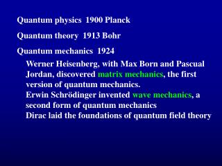
Particle in a Box (1D) - 1 ∞ ∞ V V=0 V=∞ V=∞ x 0 a Figure 11.6 Potential energy for the particle in a box. The potential (V) is zero for some finite region (0<x<a) and infinite elsewhere.
Particle in a Box (1D) - Interpretations ● Plots of Wave functions ● Plots of Squares of Wave functions ● Check Normalizations ● How fast is the particle moving? Comparison of macroscopic versus microscopic particles. Calculate v(min) of an electron in a 20-Angstrom box. Calculate v(min) of a 1 g mass in a 1 cm-box
Particle in a Box (3D) – 1 z a y a 0 a Figure 11.8 The cubic box. For the three-dimensional particle in a box, the potential is zero inside a cube and infinite elsewhere. This could represent the situation of a particle inside a container with perfectly rigid, impenetrable walls. x
Particle in a Box (3D) -Degeneracies *Energy given in units of h2/8ma2
Quantum Mechanics and Atomic Orbitals • Orbitals and Quantum Numbers