Download

1 / 47
490 likes | 706 Vues
Hop Doub lin g Label Indexing for Point-to-Point Distance Querying on Scale-Free Networks. Minhao Jiang 1 , Ada Wai-Chee Fu 2 , Raymond Chi-Wing Wong 1 , Yanyan Xu 2 The Hong Kong University of Science and Technology 1 The Chinese University of Hong Kong 2. Prepared by Minhao Jiang

E N D
Hop Doubling Label Indexing for Point-to-Point Distance Querying on Scale-Free Networks Minhao Jiang1, Ada Wai-Chee Fu2, Raymond Chi-Wing Wong1, Yanyan Xu2 The Hong Kong University of Science and Technology 1 The Chinese University of Hong Kong 2 Prepared by Minhao Jiang Presented by Minhao Jiang
Outline 1. Background 2. Our Method 3. Experiment 4. Conclusion 5. Future Work
Background 1. Point-to-Point Distance Query: Given an unweighted directed graph G = (V, E) the shortest distancedistG(u,v) from u to v in a graph G Example:distG(5,6) = 4
Background • Point-to-Point Distance Query: • Applications: • (1). Routing in communication network • (2). Social network analysis • (3). Web search • (4). Operation research • Two Approaches: • (1). Answer queries on the fly : Dijkstra's algorithm • (2). Index the graph in preprocessing and answer the query based on the index, e.g. 2-hop index.
Background 2-Hop Index: Each vertex u : 2 labels Lout (u) and Lin(u) Each label: a set of label entries (uv, d) each vertex u: querying distG(u,v) by Lout (u) and Lin(v)
Background 2. 2-Hop Index: Example:
Background 2. 2-Hop Index: querying distG(5,6) by Lout (5) and Lin(6) Example: 3+1 = 4 3+1 = 4 Solid line : graph edge label entry in the index Dotted line : created label entry
Background • Scale-Free Network: • Degree Distribution: Real Life Graphs Social Network e.g. Google plus Communication Network e.g. European email network Many real graphs can be modeled as [Science 99, SIGCOMM 99, Combinatorica 04 ,….. ] Note that some graphs are not scale-free. Scale-Free Network Web e.g. flickr.com RDF Graph e.g. Wikipedia
Background 4. Related Works: 4.1 Greedy 2-hop cover [SODA 02] • log(n)-approximation 2-hop labeling algorithm • Build 2-hop by iteratively choosing densest subgraph • Weakness: high complexity, large index size in practice (We perform well on various datasets.) 4.2 Independent-set based labeling [VLDB 13] • Build 2-hop by iteratively removing independent-set vertices • Weakness: cannot build complete 2-hop for large graphs, and querying on partial index is slow (We can build complete index and answer queries efficiently.) 4.3 Pruning landmark labeling [SIGMOD 13] • Build 2-hop by pruning labels on BFS trees • Weakness: need large memory, otherwise external BFS is inefficient for handling large disk-resident graphs (We use disk-based method to handle large disk-resident graphs efficiently.)
Background 5. Our Contribution: • Make use of the properties of scale-free graph for a distance query • Propose a novel IO-efficient method for distance query on a large disk-resident graph • Verify the performance on various large real graphs
Our Method 1. Framework: Scale-Free Networks disk-based each iteration: Label Generation 2. Pruning read write Partial Graph Partial Complete Graph + Index + Index iteratively 。 。 。 disk memory Goal 1. handle large graph disk-based IO-efficient method
Our Method Hop-Doubling Label Generation: 2.1 Properties of a Scale-Free Network Observation 1: (as black arrow) Hit most shortest paths by high-degree vertices Create labels with high-degree vertices a few high-degrees verticescan hit most long-length shortest paths Scale-Free Properties
Our Method Hop-Doubling Label Generation: 2.1 Properties of a Scale-Free Network Observation 2: (as blue arrow) Hit a few shortest paths by other vertices The number of short-length shortest paths through any vertexnot hit by high-degrees vertices is small Scale-Free Properties
Our Method Hop-Doubling Label Generation: 2.1 Properties of a Scale-Free Network There exists a 2-hop index with small size. Scale-Free Properties
Our Method • Hop-Doubling Label Generation: 2.2 Iterative Labeling Algorithm • Rank the vertices, e.g. in descending order of deg(v) Example: r(0) > r(1) > r(2) ….
Our Method • Hop-Doubling Label Generation: 2.2 Iterative Labeling Algorithm • Initialize labels with the edges • Generate labels iteratively until it can answer any query correctly
Our Method • Hop-Doubling Label Generation: 2.2 Iterative Labeling Algorithm • Generate labels based on 6 rules for each iteration
Our Method • Hop-Doubling Label Generation: 2.2 Iterative Labeling Algorithm • Generate labels based on 6 rules for each iteration Doubling effect: A length D path can be generated in iterations Example: generating (60) of length 8: Black: initialization Blue: 1st iteration Green: 2nd iteration Red: 3rd iteration
Our Method • Hop-Stepping Enhancement 3.1 Hop-Length i+1 from i and 1 Hop-Doubling: • Weakness: fast growth many labels generated Hop-Stepping Enhancement: • Strength: slower growth fewer labels generated
Our Method • Hop-Stepping Enhancement 3.2 Hop-Doubling + Hop-Stepping
Experiment • Setup: 1.1 Machine • 3.3 GHz CPU, 4GB RAM, 7200 RPM disk 1.2 Main Competitors • Baseline: bidirectional Dijkstra search • Disk-based: IS-Label [VLDB, 13] • Memory-based: PLL [SIGMOD, 13] 1.3 Datasets • Real datasets: from SNAP and KONECT • Synthetic datasets: generated by GLP model[infocom, 02]
Experiment • Performance Comparison: • IS-Label: Disk-based algorithm [VLDB, 13] • PLL: Memory-based algorithm [SIGMOD, 13] • HopDb: Disk-based algorithm [this paper]
Experiment • Performance Comparison: • BIDIJ: Memory-based bidirectional Dijkstra search • IS-Label: Disk-based algorithm [VLDB, 13] • PLL: Memory-based algorithm [SIGMOD, 13] • HopDb: Disk-based algorithm [this paper]
Experiment • Scalability: • Generate synthetic graphs by GLP model • (a). Fix |V| = 10M, varying density |E|/|V| • (b). Fix density |E|/|V|=20, varying |V|
Conclusion • HopDb can handle large graphs with limited main memory • Index building is fast • Index size is small • Very fast query time
Future Work • Handling large dynamic graph • Extending to distributed environment
END Q & A
Background 4. Our Goal: Source vertex u Destination vertex v Scale-Free Networks Index Bulding Querying distG(u,v) handle large graph disk-based IO-efficient method 2. fast indexing scale-free property for speeding up 3. small index size 2-hop index based on scale-free property 4. short query time small 2-hop index for querying
Background • 3. Scale-Free Network: • Degree distribution: • Small Diameter: • Expansion factor: Consider a BFS tree from a random vertex D: the expected height R: the expected # of branches D R
Background • 3. Scale-Free Network: • Degree distribution: • Small Diameter: • Expansion factor: • Degree deg(v), rank r(v): Example: |V|=1M, D ≈ 4.6, R ≈ 20, Degree of highest-degree vertex ≈ 63K
Examples Assumption 1: a few high-degrees vertices(e.g. v0 in the example) can hit most long-length shortest paths (e.g. all paths of length at least 4) Example: |V|=1M, v0 : the highest-degree vertex v0 is expected to reach all vertices in 2 hops, v0 is expected to hit all shortest paths ≥ 4 hops. v0
Examples Assumption 2: The number of short-length shortest paths (e.g. paths of length < 4 hops in the example) not hit by high-degrees vertices is small (e.g. 0.8%) Example: |V|=1M, v0 : the highest-degree vertex v : a random vertex without v0, v can only reach less than 0.8% vertices in < 4 hops. Shortest paths of length < 4 hops not via v0 is only 0.8%.
Examples Assumption 3: There exists a 2-hop cover with small size. (1) long-length shortest path : very likely hit by high-degree vertices (assumption 1) (2) short-length shortest path around high-degree vertices: hit by high-degree vertices (3) short-length shortest path outside high-degree vertices: very few (assumption 2)
Our Method • Hop-doubling label generation: 2.2 Iterative Labeling Algorithm • Generate labels by 6 rules iteratively correctness: w : the highest ranked vertex in a shortest path (uv) (uw) and (wv) must be generated • e.g. in shortest path (56) = (53106), • (50) and (06) are indexed
Our Method • Hop-doubling label generation: 2.2 Iterative Labeling Algorithm • Generate labels by 6 rules iteratively • e.g. in shortest path (56) = (53106), Initialization : all edges, including (53) and (06) After the 1st iteration: (51) After the 2nd iteration: (50) so (50) and (06) are generated
Our Method • Hop-Doubling Label Generation: 2.2 Iterative Labeling Algorithm • Simplify the 6 rules to 4 rules • (1)more efficient label generation • (2)still answer a distance query via the 2-hop index generated based on 4 rules
Our Method • Hop-doubling label generation: 2.2 Iterative Labeling Algorithm • Generate labels by 6 rules iteratively • In the i-th iteration, • (uv) : generated in the (i-1)-th iteration • (u1u), (u2u), (vu3): generated before the i-th iteration Doubling effect: The label length can be doubled in every 2 iterations in the worst case. A length D path can be generated in iterations, i.e. (1) Start from length 1 labels, i.e. graph edges. (2) Double label lengths every 2 iterations in the worst case. (3) IO-efficient
Our Method • Hop-doubling label generation: 2.2 Iterative Labeling Algorithm • Rank vertices by degree • Generate labels by 6 rules iteratively • rationale: • In most cases, the highest-degree vertex in one of the shortest path from a vertex to another vertex is a globally high-degree vertex(assumption 1,2,3)
Our Method • Hop-doubling label generation: 2.2 Iterative Labeling Algorithm • Rank vertices by degree • Generate labels by 6 rules iteratively • rationale:
Our Method • Triangle inequality pruning • Example: • consider (21) generated by (23) and (31), note that (21) cannot be generated by (20) and (01), • length(21) = length(231) = length(201) = 2, • Using (21), one shortest path (71) is • (72)+(21) = (7231). • Not using (21), one shortest path (71) is • (70)+(01) = (7201), • i.e. (21)=(231) can be replaced by (20) and (01)
Our Method • Triangle inequality pruning • 3.1 Iterative pruning after label generation • (uv, d) is pruned by (uw, d1) and (wv, d2) • if r(w)>r(u), r(w)>r(v) and d≥d1+d2 • any length(suvt) ≥ length(suwvt)
Our Method • Triangle-Inequality Based Pruning • IO-efficient Techniques • Details are skipped
Our Method Hop-Stepping Enhancement 3.1 Hop-Doubling VS Hop-Stepping Example: Generating (60) of length 8: 3 iterations VS 7 iterations New label entries generated: multiple VS one (in 1 iteration) Black: initialization Blue: 1st iteration Green: 2nd iteration Red: 3rd iteration Dotted Black: 4th iteration Dotted Blue: 5th iteration Dotted Green: 6th iteration Dotted Red: 7th iteration
Our Method • Hop-Stepping enhancement 4.1 Hop-length i+1 from i and 1 Hop-doubling: • hop-length i : (uv), (u1u), (u2u), (vu4), (vu5) Hop-stepping: • hop-length i : (uv) • hop-length 1 : (u1u), (u2u), (vu4), (vu5) • Correctness still holds • more iterations
Our Method • IO-efficient implementation 5.1 IO-efficient label generation • Take rule 1 & 2 as an example: • Block nested loop by rule 1 & 2 simultaneously: • Load the labels in the following order for IO-efficient • (1). Outer loop (u*) and (*u): • (uv), (uv’), (uv’’), ... (u1u), (u1’u), (u1’’u), ... • (2). Inner loop (u2*): • (u2u), (u2u’), (u2u’’), ...
Our Method • IO-efficient implementation 5.1 IO-efficient label generation • Block nested loop: Current inner block Current outer block Next inner block Next outer block
Our Method • IO-efficient implementation 5.2 IO-efficient pruning • Take when r(w)>r(v)>r(u) as an example • Block nested loop: • Load the labels in the following order for IO-efficient • (1). Outer loop (u*): • (uw), (uw’), (uw’’), … (uv), (uv’), (uv’’), … (2). Inner loop (*v): (wv), (w’v), (w’’v), …