Download
1 / 69
740 likes | 1.12k Vues
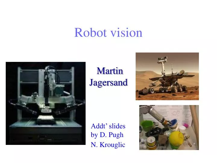
Robot vision. Martin Jagersand. Addt’ slides by D. Pugh N. Krouglic. What is Computer Vision?. Computer Vision. Computer Vision. Computer Graphics. Image Processing. Three Related fields Image Processing: Changes 2D images into other 2D images

E N D
Robot vision Martin Jagersand Addt’ slides by D. Pugh N. Krouglic
What is Computer Vision? Computer Vision Computer Vision Computer Graphics Image Processing • Three Related fields • Image Processing: Changes 2D images into other 2D images • Computer Graphics: Takes 3D models, renders 2D images • Computer vision: Extracts scene information from 2D images and video • e.g. Geometry, “Where” something is in 3D, • Objects “What” something is” • What information is in a 2D image? • What information do we need for 3D analysis? • CV hard. Only special cases can be solved. 90 horizon
Machine Vision • 3D Camera vision in general environments hard • Machine vision: • Use engineered environment • Use 2D when possible • Special markers/LED • Can buy working system! • Photogrammetry: • Outdoors • 3D surveying using cameras
Vision v u Y X • Full: Human vision • We don’t know how it works in detail • Limited vision: Machines, Robots, “AI” What is the most basic useful information we can get from a camera? • Location of a dot (LED/Marker) [u,v] = f(I) • Segmentation of object pixels All of these are 2D image plane measurements! What is the best camera location? Usually overhead pointing straight down Adjust cam position so pixel [u,v] = s[X,Y]. Pixel coordinates are scaled world coord
Tracking LED special markers v u Y X • Put camera overhead pointing straight down on worktable. • Adjust cam position so pixel [u,v] = s[X,Y]. Pixel coordinates are scaled world coord • Lower brightness so LED brighterest • Put LED on robot end-effector • Detection algorithm: • Threshold brightest pixels I(u,v)>200 • Find centroid [u,v] of max pixels • Variations: • Blinking LED can enhance detection in ambient light. • Different color LED’s can be detected separately from R,G,B color video. Camera LED
Commercial tracking systems Polaris Vicra infra-red system(Northern Digitial Inc.) MicronTracker visible light system (Claron Technology Inc.)
Commercial tracking system Images acquired by the Polaris Vicra infra-red stereo system: right image left image
IMAGE SEGMENTATION • How many “objects” are there in the image below? • Assuming the answer is “4”, what exactly defines an object? Zoom In 8/31/2014 Introduction to Machine Vision
8 BIT GRAYSCALE IMAGE 8/31/2014 Introduction to Machine Vision
8 BIT GRAYSCALE IMAGE 8/31/2014 Introduction to Machine Vision
Compare: Natural image What is this? 207 200 194 194 203 130 105 095 107 153 192 196 190 186 175 242 194 222 254 255 124 074 082 072 076 208 206 202 194 185 254 170 204 255 248 122 153 135 111 081 252 253 233 232 250 255 172 201 255 249 123 092 040 094 106 255 253 239 150 254 255 197 192 255 248 133 024 027 076 032 250 255 255 181 255 253 210 190 239 250 089 092 149 128 013 254 254 253 229 255 252 238 180 218 251 106 116 181 140 024 250 255 255 255 200 248 248 169 227 252 111 066 118 061 021 252 251 255 255 142 253 255 171 254 253 142 037 132 006 017 253 253 255 254 201 253 250 170 255 253 139 134 127 156 078 255 253 253 254 237 254 228 169 213 235 146 123 096 090 130 230 250 253 254 254 252 244 140 215 245 125 055 043 081 077 252 234 253 253 253 254 250 169 211 235 117 108 093 119 078 246 249 235 225 255 254 234 167 212 217 110 070 049 098 074 244 246 239 207 254 255 219 170 238 253 113 130 109 063 075 243 235 233 252 252 255 221 179 248 227 111 083 041 061 083 240 249 243 232 253 221 217 180 213 243 109 079 048 100 045 246 249 244 221 210 236 216 178 208 230 156 077 062 110 088 244 249 230 220 221 229 224 183 211 132 052 087 062 124 085 135 246 236 220 214 230 223 185 185 112 079 008 124 158 125 119 119 232 225 232 221 215 194 100 154 071 008 031 097 010 093 098 148 229 216 223 217 132 046 072 076 056 048 013 182 073 076 083 215 219 224 216 041 102 090 162 079 111 118 164 083 170 065 221 219 215 222 046 111 077 075 060 046 069 032 179 068 157 224 226 219 216 092 045 074 143 013 171 159 072 087 065 143 217 222 222 224 070 041 074 131 085 150 112 140 139 154 055 231 218 226 232 118 109 041 165 130 105 097 175 078 081 067 064 174 253 254 079 072 116 089 020 068 103 074 031 130 106 052 161 047 034 090 045 145 027 135 109 082 082 048 113 087 061 157 193 192 057 038 051 092 018 062 110 052 060 084 066 071 154 191 192 043 153 052 030 078 061 062 054 046 049 054 078 158 184 181 066 019 043 038 046 083 057 050 145 048 035 087 158 138 074 030 082 030 038 076 041 141 046 045 040 009 063 149 135 016 057 071 035 025 040 062 030 084 130 043 059 113 151
Compare: Natural image 020 067 073 058 055 076 069 050 074 064 065 066 066 059 023 047 109 107 118 107 115 110 120 120 124 120 128 124 132 131 047 125 130 130 122 121 117 142 131 133 134 141 149 144 135 051 139 143 139 147 134 149 069 127 144 139 144 150 161 149 054 136 161 148 147 158 055 052 034 030 158 156 165 163 156 043 144 165 159 154 171 224 191 047 030 171 165 175 164 163 025 161 174 172 167 049 200 193 112 028 120 169 173 177 173 011 091 101 105 177 039 078 060 041 026 073 102 167 208 121 011 091 094 066 094 033 199 184 139 024 060 094 125 152 134 009 068 072 072 065 031 151 171 075 028 035 072 083 109 063 013 068 074 059 057 037 161 129 062 028 035 071 072 078 056 012 042 063 055 072 033 020 067 031 022 027 082 070 073 060 011 037 064 094 091 026 025 080 066 026 023 071 070 080 060 011 060 077 082 037 023 024 147 140 038 023 037 043 076 037 013 049 076 059 032 028 174 197 182 060 021 021 121 101 062 013 059 111 072 020 078 200 211 182 061 069 059 043 086 106 007 053 057 092 023 105 189 230 210 084 034 021 017 033 091 011 061 072 018 027 054 069 068 062 023 045 011 016 042 044 014 041 047 025 018 040 065 039 024 021 036 041 013 030 022 013 093 106 017 019 027 030 042 012 021 043 013 014 020 027 019 040 029 023 016 024 015 026 011 010 026 017 012 013 014 022 042 030 040 019 015 016 011 012 009 008 012 009 017 019 022 026 018 030 020 012 017 010 008 011 007 015 008 016 034 019 018 048 029 012 054 012 008 008 009 008 012 007 016 005 022 015 057 043 126 135 122 006 005 008 007 019 010 011 008 018 008 009 019 023 093 109 128 063 052 031 010 012 009 006 017 010 010 007 067 054 106 116 067 056 011 028 005 009 006 015 010 012 014 062 076 057 055 019 024 020 006 005 013 004 016 010 008 011 039 025 020 016 011 007 008 007 006 010 003 015 009 010 010 012 011 014 009 008 007 007 005 005 008 002 014 007 008 011 007 012 010 009 007 008 007 005 005 007 003 020 011 015 019 013 017 017 013 019 013 012 013 011 009 005 020 067 073 058 055 076 069 050 074 064 065 066 066 059 023 025 161 174 172 167 049 200 193 112 028 120 169 173 177 173
GRAY LEVEL THRESHOLDING • Many images consist of two regions that occupy different gray level ranges. • Such images are characterized by a bimodal image histogram. • An image histogram is a function h defined on the set of gray levels in a given image. • The value h(k) is given by the number of pixels in the image having image intensity k. 8/31/2014 Introduction to Machine Vision
GRAY LEVEL THRESHOLDING Objects Set threshold here 8/31/2014 Introduction to Machine Vision
BINARY IMAGE 8/31/2014 Introduction to Machine Vision
IMAGE SEGMENTATION – CONNECTED COMPONENT LABELING • Segmentation can be viewed as a process of pixel classification; the image is segmented into objects or regions by assigning individual pixels to classes. • Connected Component Labeling assigns pixels to specific classes by verifying if an adjoining pixel (i.e., neighboring pixel) already belongs to that class. • There are two “standard” definitions of pixel connectivity: 4 neighbor connectivity and 8 neighbor connectivity. 8/31/2014 Introduction to Machine Vision
IMAGE SEGMENTATION – CONNECTED COMPONENT LABELING 4 Neighbor Connectivity 8 Neighbor Connectivity 8/31/2014 Introduction to Machine Vision
CONNECTED COMPONENT LABELING: FIRST PASS A A EQUIVALENCE: B=C A A A B B C C B B B C C B B B B B B 8/31/2014 Introduction to Machine Vision
CONNECTED COMPONENT LABELING: SECOND PASS A A TWO OBJECTS! A A A B B B C C B B B B B C B C B B B B B B 8/31/2014 Introduction to Machine Vision
CONNECTED COMPONENT LABELING: TABLE OF EQUIVALENCES 8/31/2014 Introduction to Machine Vision
CONNECTED COMPONENT LABELING: TABLE OF EQUIVALENCES 8/31/2014 Introduction to Machine Vision
IS THERE A MORE COMPUTATIONALLY EFFICIENT TECHNIQUE FOR SEGMENTING THE OBJECTS IN THE IMAGE? • Contour tracking/border following identify the pixels that fall on the boundaries of the objects, i.e., pixels that have a neighbor that belongs to the background class or region. • There are two “standard” code definitions used to represent boundaries: code definitions based on 4-connectivity (crack code) and code definitions based on 8-connectivity (chain code). 8/31/2014 Introduction to Machine Vision
BOUNDARY REPRESENTATIONS: 4-CONNECTIVITY (CRACK CODE) CRACK CODE: 10111211222322333300103300 8/31/2014 Introduction to Machine Vision
BOUNDARY REPRESENTATIONS: 8-CONNECTIVITY (CHAIN CODE) CHAIN CODE: 12232445466601760 8/31/2014 Introduction to Machine Vision
CONTOUR TRACKING ALGORITHM FOR GENERATING CRACK CODE • Identify a pixel P that belongs to the class “objects” and a neighboring pixel (4 neighbor connectivity) Q that belongs to the class “background”. • Depending on the relative position of Q relative to P, identify pixels U and V as follows: 8/31/2014 Introduction to Machine Vision
CONTOUR TRACKING ALGORITHM • Assume that a pixel has a value of “1” if it belongs to the class “object” and “0” if it belongs to the class “background”. • Pixels U and V are used to determine the next “move” (i.e., the next element of crack code) as summarized in the following truth table: 8/31/2014 Introduction to Machine Vision
CONTOUR TRACKING ALGORITHM V Q P U Q V P U V Q U P V Q U P V U 8/31/2014 Introduction to Machine Vision
CONTOUR TRACKING ALGORITHM FOR GENERATING CHAIN CODE • Identify a pixel P that belongs to the class “objects” and a neighboring pixel (4 neighbor connectivity) R0 that belongs to the class “background”. Assume that a pixel has a value of “1” if it belongs to the class “object” and “0” if it belongs to the class “background”. • Assign the 8-connectivity neighbors of P to R0, R1, …, R7 as follows: 8/31/2014 Introduction to Machine Vision
CONTOUR TRACKING ALGORITHM FOR GENERATING CHAIN CODE • ALGORITHM: • i=0 • WHILE (Ri==0) { i++ } • Move P to Ri • Set i=6 for next search 8/31/2014 Introduction to Machine Vision
OBJECT RECOGNITION – BLOB ANALYSIS • Once the image has been segmented into classes representing the objects in the image, the next step is to generate a high level description of the various objects. • A comprehensive set of form parameters describing each object or region in an image is useful for object recognition. • Ideally the form parameters should be independent of the object’s position and orientation as well as the distance between the camera and the object (i.e., scale factor). 8/31/2014 Introduction to Machine Vision
What are some examples of form parameters that would be useful in identifying the objects in the image below? 8/31/2014 Introduction to Machine Vision
OBJECT RECOGNITION – BLOB ANALYSIS • Examples of form parameters that are invariant with respect to position, orientation, and scale: • Number of holes in the object • Compactness or Complexity: (Perimeter)2/Area • Moment invariants • All of these parameters can be evaluated during contour following. 8/31/2014 Introduction to Machine Vision
GENERALIZED MOMENTS • Shape features or form parameters provide a high level description of objects or regions in an image • Many shape features can be conveniently represented in terms of moments. The (p,q)th moment of a region R defined by the function f(x,y) is given by: 8/31/2014 Introduction to Machine Vision
GENERALIZED MOMENTS • In the case of a digital image of size n by m pixels, this equation simplifies to: • For binary images the function f(x,y) takes a value of 1 for pixels belonging to class “object” and “0” for class “background”. 8/31/2014 Introduction to Machine Vision
GENERALIZED MOMENTS X 7 Area 33 20 159 Moment of Inertia 64 93 Y 8/31/2014 Introduction to Machine Vision
SOME USEFUL MOMENTS • The center of mass of a region can be defined in terms of generalized moments as follows: 8/31/2014 Introduction to Machine Vision
SOME USEFUL MOMENTS • The moments of inertia relative to the center of mass can be determined by applying the general form of the parallel axis theorem: 8/31/2014 Introduction to Machine Vision
SOME USEFUL MOMENTS • The principal axis of an object is the axis passing through the center of mass which yields the minimum moment of inertia. • This axis forms an angle θ with respect to the X axis. • The principal axis is useful in robotics for determining the orientation of randomly placed objects. 8/31/2014 Introduction to Machine Vision
Example X Principal Axis Center of Mass Y 8/31/2014 Introduction to Machine Vision
SOME (MORE) USEFUL MOMENTS • The minimum/maximum moment of inertia about an axis passing through the center of mass are given by: 8/31/2014 Introduction to Machine Vision
SOME (MORE) USEFUL MOMENTS • The following moments are independent of position, orientation, and reflection. They can be used to identify the object in the image. 8/31/2014 Introduction to Machine Vision
SOME (MORE) USEFUL MOMENTS • The following moments are normalized with respect to area. They are independent of position, orientation, reflection, and scale. 8/31/2014 Introduction to Machine Vision
EVALUATING MOMENTS DURING CONTOUR TRACKING • Generalized moments are computed by evaluating a double (i.e., surface) integral over a region of the image. • The surface integral can be transformed into a line integral around the boundary of the region by applying Green’s Theorem. • The line integral can be easily evaluated during contour tracking. • The process is analogous to using a planimeter to graphically evaluate the area of a geometric figure. 8/31/2014 Introduction to Machine Vision
3D MACHINE VISION SYSTEM XY Table Laser Projector Digital Camera Field of View Plane of Laser Light Granite Surface Plate P(x,y,z) 8/31/2014 Introduction to Machine Vision
3D MACHINE VISION SYSTEM 8/31/2014 Introduction to Machine Vision
3D MACHINE VISION SYSTEM 8/31/2014 Introduction to Machine Vision
3D MACHINE VISION SYSTEM 8/31/2014 Introduction to Machine Vision
3D MACHINE VISION SYSTEM 8/31/2014 Introduction to Machine Vision
Commercial Machine VisionDefinition “Machine vision is the capturing of an image (a snapshot in time), the conversion of the image to digital information, and the application of processing algorithms to extract useful information about the image for the purposes of pattern recognition, part inspection, or part positioning and orientation”….Ed Red
Current State Cheap and Easy to Use • The Sony approved Scorpion Robot Inspection Starter Kit contains everything you need for bringing your Scorpion Robot Inspection project to life. • The kit includes a Scorpion Enterprise software license • new high quality Sony XCD-710 (CR) camera (XGA resolution) • Sony Desktop Robot • 2 days training course • A standard and configurable user interface paired with innovative, easy-to-use and robust imaging tools • $1995.00