Download

1 / 40
420 likes | 813 Vues
Instrumental Variables. Saralyn J Miller EDU 7314. Overview of Presentation. Understanding IV History Defined Assumptions Endogeneity Exogenous Variable - Instrument Angrist example paralleled with an education example Statistical Understanding of IV Present 2 equations Card Example

E N D
Instrumental Variables Saralyn J Miller EDU 7314
Overview of Presentation • Understanding IV • History • Defined • Assumptions • Endogeneity • Exogenous Variable - Instrument • Angrist example paralleled with an education example • Statistical Understanding of IV • Present 2 equations • Card Example • Overview of article • Replicate his study in R • In-class Example • Other Examples of IV in Education
History of IV • Historically IV has mostly been used by economists and statisticians (Angrist & Kreuger, 2001). • Philip G. Wright (econometrician) vs. Sewell Wright (biologist) (Wright, 1928). • Philip had written about the problem of endogenous variation in previous papers. • Sewell had discovered the use of an instrument, but the variables were already exogenous, so the analysis was unnecessary. • Stylometric analysis of their writing (Stock & Trebbi, 2003 • Authors found Philip to be the writer and founder of IV • 1940’s IV was rediscovered • 1953 Theil introduced the two stage least squares method for computing IV
Instrumental Variables Defined • Causality is difficult to prove, even in experimental research. • In education, randomization is what is used to determine causality. • However, we can’t always randomize or create a true experiment. • The IV method is a quasi-experimental research method used to estimate causal relationships.
Regression Assumption • One of the assumptions of the error term in a regression analysis is that the error must be independent and identically distributed. • Error variance is the same for all values. • Error is not related to other error values. • Error is normally distributed. • Use IV when the independent variable is correlated with unobservable error. • 3 reasons why this assumption might be violated: • Omitted variable bias: When an unobservable variable is capturing some of the dependent variable and this unobservable variable is not in your model. Instead, the variables you have included are picking up some of the unobserved and the unobserved needs to be accounted for on it’s own. In other words, there are other variables that can explain the outcome measure and your variable is picking up some of this explanation (omitted variable bias). • Measurement error – causation is not determined due to error in the collection of the data • Reverse Causality – direction of causality is not determined. http://www.unescap.org/tid/artnet/mtg/gravity_d4s1_shepherd.pdf
Endogeneity • When an independent variable correlates with unobservable error we call this endogeneity. • Endogenous variables: variables that are correlated with error term. You can’t say that the independent variables cause the dependent variable. • Often the factors that affect an outcome depend on that outcome (reverse causality). • Example • The more shots Kobe Bryant takes, the lower the percentage of wins for the Lakers. Does an increase in shots that Kobe takes cause the Lakers to lose? Or does the loss of the game and the fact that teammates are not making shots cause Kobe to take more shots? (http://drbseconomicblog.blogspot.com/2009/01/kobe-and-reverse-causality.html )
Endogeneity • Sometimes in a linear model some of the variables are endogenous, meaning the regressors or variables are correlated with the error term. • Ex: Effect of military service on future earnings (Angrist, 1990). • Military service is endogenous. • Does the military cause a soldier’s future earnings to be a certain amount when he or she leaves the service? Or are there certain characteristics of those that join the military that influence future earnings? • An individual’s choice to enter the service might be indicative of the individual’s expected future earnings. There are some individuals that choose to go into the military because their expected future earnings are low. Therefore, their enrollment is related to the fact that those that join the service might on average have lower future earnings. • Also, veterans have certain observed and unobserved characteristics that affect their decision to enroll and these could be related to earnings. http://financialaccess.org/node/2042
What do we do when you have an endogenous variable? • An exogenous variable or instrument can “fix” endogeneity. • These variables are correlated with the regressors, but are uncorrelated with the error term. • We call these exogenous variables instruments. • Ex: Since determining earnings is dependent on other things such as expected earnings, Angrist (1990) used the Vietnam draft as an instrument. It is correlated with entering the service, but is not correlated with earnings. The draft system is exogenous.
Qualities of an Instrument – Exogenous Variable • It must be correlated with the independent variable. • It must be uncorrelated with the error of the dependent variable. • Assumption of IV: Instrument must be exogenous.
Example • Joshua Angrist’s 1990 work. • He analyzed the difference in earnings between veterans and non-veterans. • But analyzing this difference does not tell us the causal impact of military service on future earnings. • In education – we “fix” this problem by randomly placing students into treatment and control conditions. • We can’t always randomize. What if we gave students a choice on whether they wanted to attend tutoring sessions (Reardon, 2010) because we could not randomly assign students to a condition?
Example Continued • A young person’s decision to enter the military could be affected by his/her expectations of future earnings. This is an endogeneity problem: does military service affect future earnings or does the prospect of future earnings affect the decision to enter the military? • Veterans have observed and unobserved characteristics that affect their reason for entering the military. We cannot control for the unobserved characteristics. • Tutoring session example (Reardon, 2010): A student’s decision to attend tutoring could be affected by his/her expectations of how it will affect academic achievement. Does tutoring affect achievement or does the prospect of future grades affect the decision to go to tutoring?
What did Angrist do? • He used the Vietnam draft lottery as an instrument (exogenous variable). • The draft lottery is correlated with serving in the military. • The draft lottery is only correlated with future earnings of military personnel through enrollment in the military. • Tutoring session could use a lottery system too. • The lottery would be correlated with those that go to tutoring. • The lottery would be correlated with future grades only through attendance to the tutoring program.
Problem • What about those who were drafted and avoided the draft? • Or those who were not drafted, but felt compelled to fight anyway? • What about the students who were picked for the lottery, but chose not to go because they didn’t think it would help? • Or those that were not picked, but really felt like they needed the help?
Answer • The IV method recognizes that those described previously cannot be included in the sample. It is not an average treatment effect for the whole sample, but is a local average treatment effect (LATE) • Military earnings example only tells you the treatment effect on those who pulled a “bad” number and served and those who pulled a “good” number and did not serve. • Tutoring example: only tells you the treatment effect on those who were picked for tutoring and attended and those who were not picked for tutoring and did not attend. • Therefore we are only measuring a treatment effect for compliers, which makes this method less generalizable.
IV Limitations & Advantages • Limitations • LATE • Estimates can be biased when not a binary choice, but an ordered choice (use LIV to correct). • There is not usually a theoretical model that the relationships are based on except when a natural experiment is created. • Only generalizable to those that benefit from the instrument. • Advantages • Can be used to estimate a causal relationship when randomization is not applicable.
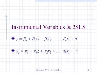
Statistical Understanding of IV • Think of IV models as 2 separate equations. • Y is the outcome variable • K is the variable related to the instrument • IV is the instrument related to K • e is the error
Typical Regression Endogenous Exogenous X1 e1 DV X2
Instrumental Variable Regression Exogenous Instrumental Variable Endogenous Exogenous X1 e1 X2
How do we find a good instrument and test the instrument’s validity? • You can use theory and past research to provide evidence for an instrument. • Hausman test • Check correlation between independent variable and instrument.
Example in R – Card data • Explanation of Card (1993) study • Replicate study using Card data (Card, 1993; Hamersma, 2009).
Using Geographic Variation in College Proximity to Estimate the Return to Schooling (Card, 1993) • Does level of education or number of years of schooling effect wages or earnings? • You would think yes! • BUT, the studies that show earnings gains are controversial because educational levels are NOT randomly assigned. Individuals choose their level of education. Education is endogenous. • The effect of schooling is difficult to determine and you cannot randomly assign some children to school. • The author needs an exogenous variable. Card uses geographic differences in the proximity to a college. • Overall finding: When college proximity is used as an instrument in place of education, the author finds that the return to education is approximately 50% higher than the OLS estimate.
Why is Education Endogenous to Earnings? • Ability bias – if some individuals have an ability that explains earnings despite education, then those that earn higher schooling will have an upward-biased level of earnings (IQ). • Measurement error- All of the data was student reported. We could argue that there is a negative correlation between earnings error and observed schooling.
Is College Proximity Exogenous? • Card proposes college proximity as an exogenous variable. College proximity needs to be related to wages, but only through education. • If you are poor, the likelihood of attending college increases if you live near one, so proximity is related to education. • He checked this by looking at the effect of college proximity on predicted education given other demographic variables. Biggest effect was men with low chance of continuing education. (if you live near a college, then there is a lower cost of higher education so there is a bigger effect on education outcomes of poorer children)
Recap • We’re trying to predict the effect of schooling on wages. • Education is our key independent variable that is endogenous. • Wage (log of wages) is our dependent variable. • College proximity is our exogenous instrument.
Variables Used in Card analysis • lwage = log(wages) • educ = years of schooling, 1976 • exper = age – educ – 6 • expersq • black = 1 if black • south = 1 if in south, 1976 • smsa = 1 if in metropolitan area, 1976 • reg661-reg668 = 1 for region lived in, 1966 • smsa66 = 1 if in metropolitan area, 1966 • nearc4 = 1 if near 4 year college, 1966
3 Step Process for Replicating Card’s Findings (Card, 1992; Hamersma, 2009) ###Load Stata file### library(foreign) card.data<-read.dta("card.dta") attach(card.data) head(card.data) id nearc2 nearc4 educ age fatheducmotheduc weight momdad14 sinmom14 step14 1 2 0 0 7 29 NA NA 158413 1 0 0 2 3 0 0 12 27 8 8 380166 1 0 0 3 4 0 0 12 34 14 12 367470 1 0 0 4 5 1 1 11 27 11 12 380166 1 0 0 5 6 1 1 12 34 8 7 367470 1 0 0 6 7 1 1 12 26 9 12 380166 1 0 0 reg661 reg662 reg663 reg664 reg665 reg666 reg667 reg668 reg669 south66 black 1 1 0 0 0 0 0 0 0 0 0 1 2 1 0 0 0 0 0 0 0 0 0 0 3 1 0 0 0 0 0 0 0 0 0 0 4 0 1 0 0 0 0 0 0 0 0 0 5 0 1 0 0 0 0 0 0 0 0 0 6 0 1 0 0 0 0 0 0 0 0 0 smsa south smsa66 wage enroll kwwiq married libcrd14 experlwageexpersq 1 1 0 1 548 0 15 NA 1 0 16 6.306275 256 2 1 0 1 481 0 35 93 1 1 9 6.175867 81 3 1 0 1 721 0 42 103 1 1 16 6.580639 256 4 1 0 1 250 0 25 88 1 1 10 5.521461 100 5 1 0 1 729 0 34 108 1 0 16 6.591674 256 6 1 0 1 500 0 38 85 1 1 8 6.214608 64
Step 1: OLS Estimate without InstrumentWe find education is SSD, but we can make the case that it is endogenous. m1<-lm(lwage~educ+exper+expersq+black+south+smsa+reg661+reg662+reg663+reg664+reg665+reg666+reg667+reg668+smsa66) summary(m1) Call: lm(formula = lwage ~ educ + exper + expersq + black + south + smsa + reg661 + reg662 + reg663 + reg664 + reg665 + reg666 + reg667 + reg668 + smsa66) Residuals: Min 1Q Median 3Q Max -1.62326 -0.22141 0.02001 0.23932 1.33340 Coefficients: Estimate Std. Error t value Pr(>|t|) (Intercept) 4.7393766 0.0715282 66.259 < 2e-16 *** educ 0.0746933 0.0034983 21.351 < 2e-16 *** exper 0.0848320 0.0066242 12.806 < 2e-16 *** expersq -0.0022870 0.0003166 -7.223 6.41e-13 *** black -0.1990123 0.0182483 -10.906 < 2e-16 *** south -0.1479550 0.0259799 -5.695 1.35e-08 *** smsa 0.1363845 0.0201005 6.785 1.39e-11 *** reg661 -0.1185698 0.0388301 -3.054 0.002281 ** reg662 -0.0222026 0.0282575 -0.786 0.432092 reg663 0.0259703 0.0273644 0.949 0.342670 reg664 -0.0634942 0.0356803 -1.780 0.075254 . reg665 0.0094551 0.0361174 0.262 0.793503 reg666 0.0219476 0.0400984 0.547 0.584182 reg667 -0.0005887 0.0393793 -0.015 0.988073 reg668 -0.1750058 0.0463394 -3.777 0.000162 *** smsa66 0.0262417 0.0194477 1.349 0.177327 --- Signif. codes: 0 ‘***’ 0.001 ‘**’ 0.01 ‘*’ 0.05 ‘.’ 0.1 ‘ ’ 1 Residual standard error: 0.3723 on 2994 degrees of freedom Multiple R-squared: 0.2998, Adjusted R-squared: 0.2963 F-statistic: 85.48 on 15 and 2994 DF, p-value: < 2.2e-16
What do we know so far? • Education is the key variable and is SSD, but education is endogenous and is not accounting for individual ability. • Card uses college proximity as an instrument to correct endogenous scenario. College proximity is correlated with wages, but only through education • We want to check to see if college proximity is correlated with education.
Step 2: Is college proximity an exogenous determinant of wages? m2<-lm(educ~exper+expersq+black+south+smsa+reg661+reg662+reg663+reg664+reg665+reg666+reg667+reg668+smsa66+nearc4) summary(m2) Call: lm(formula = educ ~ exper + expersq + black + south + smsa + reg661 + reg662 + reg663 + reg664 + reg665 + reg666 + reg667 + reg668 + smsa66 + nearc4) Residuals: Min 1Q Median 3Q Max -7.54513 -1.36996 -0.09103 1.27836 6.23847 Coefficients: Estimate Std. Error t value Pr(>|t|) (Intercept) 16.8485239 0.2111222 79.805 < 2e-16 *** exper -0.4125334 0.0336996 -12.241 < 2e-16 *** expersq 0.0008686 0.0016504 0.526 0.598728 black -0.9355287 0.0937348 -9.981 < 2e-16 *** south -0.0516126 0.1354284 -0.381 0.703152 smsa 0.4021825 0.1048112 3.837 0.000127 *** reg661 -0.2102710 0.2024568 -1.039 0.299076 reg662 -0.2889073 0.1473395 -1.961 0.049992 * reg663 -0.2382099 0.1426357 -1.670 0.095012 . reg664 -0.0930890 0.1859827 -0.501 0.616742 reg665 -0.4828875 0.1881872 -2.566 0.010336 * reg666 -0.5130857 0.2096352 -2.448 0.014442 * reg667 -0.4270887 0.2056208 -2.077 0.037880 * reg668 0.3136204 0.2416739 1.298 0.194490 smsa66 0.0254805 0.1057692 0.241 0.809644 nearc4 0.3198989 0.0878638 3.641 0.000276 *** --- Signif. codes: 0 ‘***’ 0.001 ‘**’ 0.01 ‘*’ 0.05 ‘.’ 0.1 ‘ ’ 1 Residual standard error: 1.941 on 2994 degrees of freedom Multiple R-squared: 0.4771, Adjusted R-squared: 0.4745 F-statistic: 182.1 on 15 and 2994 DF, p-value: < 2.2e-16
Step 2: Is college proximity an exogenous determinant of wages? m3<-lm(lwage~exper+expersq+black+south+smsa+reg661+reg662+reg663+reg664+reg665+reg666+reg667+reg668+smsa66+nearc4) summary(m3) Call: lm(formula = lwage ~ exper + expersq + black + south + smsa + reg661 + reg662 + reg663 + reg664 + reg665 + reg666 + reg667 + reg668 + smsa66 + nearc4) Residuals: Min 1Q Median 3Q Max -1.57387 -0.25161 0.01483 0.27229 1.38522 Coefficients: Estimate Std. Error t value Pr(>|t|) (Intercept) 5.9896107 0.0434375 137.890 < 2e-16 *** exper 0.0540214 0.0069336 7.791 9.07e-15 *** expersq -0.0022207 0.0003396 -6.540 7.21e-11 *** black -0.2698014 0.0192855 -13.990 < 2e-16 *** south -0.1514588 0.0278638 -5.436 5.90e-08 *** smsa 0.1646968 0.0215645 7.637 2.96e-14 *** reg661 -0.1354657 0.0416546 -3.252 0.00116 ** reg662 -0.0450389 0.0303145 -1.486 0.13746 reg663 0.0091190 0.0293467 0.311 0.75602 reg664 -0.0701587 0.0382651 -1.833 0.06683 . reg665 -0.0250439 0.0387187 -0.647 0.51780 reg666 -0.0123840 0.0431315 -0.287 0.77404 reg667 -0.0294058 0.0423056 -0.695 0.48706 reg668 -0.1496489 0.0497234 -3.010 0.00264 ** smsa66 0.0218819 0.0217616 1.006 0.31472 nearc4 0.0420679 0.0180776 2.327 0.02003 * --- Signif. codes: 0 ‘***’ 0.001 ‘**’ 0.01 ‘*’ 0.05 ‘.’ 0.1 ‘ ’ 1 Residual standard error: 0.3993 on 2994 degrees of freedom Multiple R-squared: 0.1947, Adjusted R-squared: 0.1907 F-statistic: 48.25 on 15 and 2994 DF, p-value: < 2.2e-16
Step 3: Does education effect wages when college proximity is used as the instrument? library(AER) m4<-ivreg(lwage~educ+exper+expersq+black+south+smsa+reg661+reg662+reg663+reg664+reg665+reg666+reg667+reg668+smsa66|nearc4+exper+expersq+black+south+smsa+reg661+reg662+reg663+reg664+reg665+reg666+reg667+reg668+smsa66) summary(m4) Call: ivreg(formula = lwage ~ educ + exper + expersq + black + south + smsa + reg661 + reg662 + reg663 + reg664 + reg665 + reg666 + reg667 + reg668 + smsa66 | nearc4 + exper + expersq + black + south + smsa + reg661 + reg662 + reg663 + reg664 + reg665 + reg666 + reg667 + reg668 + smsa66) Residuals: Min 1Q Median 3Q Max -1.83164 -0.24075 0.02428 0.25208 1.42760 Coefficients: Estimate Std. Error t value Pr(>|t|) (Intercept) 3.7739651 0.9349470 4.037 5.56e-05 *** educ 0.1315038 0.0549637 2.393 0.016793 * exper 0.1082711 0.0236586 4.576 4.92e-06 *** expersq -0.0023349 0.0003335 -7.001 3.12e-12 *** black -0.1467757 0.0538999 -2.723 0.006504 ** south -0.1446715 0.0272846 -5.302 1.23e-07 *** smsa 0.1118083 0.0316620 3.531 0.000420 *** reg661 -0.1078142 0.0418137 -2.578 0.009972 ** reg662 -0.0070465 0.0329073 -0.214 0.830460 reg663 0.0404445 0.0317806 1.273 0.203252 reg664 -0.0579172 0.0376059 -1.540 0.123640 reg665 0.0384577 0.0469387 0.819 0.412671 reg666 0.0550887 0.0526597 1.046 0.295587 reg667 0.0267580 0.0488287 0.548 0.583735 reg668 -0.1908912 0.0507113 -3.764 0.000170 *** smsa66 0.0185311 0.0216086 0.858 0.391193 --- Signif. codes: 0 ‘***’ 0.001 ‘**’ 0.01 ‘*’ 0.05 ‘.’ 0.1 ‘ ’ 1 Residual standard error: 0.3883 on 2994 degrees of freedom Multiple R-Squared: 0.2382, Adjusted R-squared: 0.2343 Wald test: 51.01 on 15 and 2994 DF, p-value: < 2.2e-16
Compare OLS to IV Estimator lm(formula = lwage ~ educ + exper + expersq + black + south + smsa + reg661 + reg662 + reg663 + reg664 + reg665 + reg666 + reg667 + reg668 + smsa66) Residuals: Min 1Q Median 3Q Max -1.62326 -0.22141 0.02001 0.23932 1.33340 Coefficients: Estimate Std. Error t value Pr(>|t|) (Intercept) 4.7393766 0.0715282 66.259 < 2e-16 *** educ 0.0746933 0.0034983 21.351 < 2e-16 *** exper 0.0848320 0.0066242 12.806 < 2e-16 *** expersq -0.0022870 0.0003166 -7.223 6.41e-13 *** black -0.1990123 0.0182483 -10.906 < 2e-16 *** south -0.1479550 0.0259799 -5.695 1.35e-08 *** smsa 0.1363845 0.0201005 6.785 1.39e-11 *** reg661 -0.1185698 0.0388301 -3.054 0.002281 ** reg662 -0.0222026 0.0282575 -0.786 0.432092 reg663 0.0259703 0.0273644 0.949 0.342670 reg664 -0.0634942 0.0356803 -1.780 0.075254 . reg665 0.0094551 0.0361174 0.262 0.793503 reg666 0.0219476 0.0400984 0.547 0.584182 reg667 -0.0005887 0.0393793 -0.015 0.988073 reg668 -0.1750058 0.0463394 -3.777 0.000162 *** smsa66 0.0262417 0.0194477 1.349 0.177327 --- Signif. codes: 0 ‘***’ 0.001 ‘**’ 0.01 ‘*’ 0.05 ‘.’ 0.1 ‘ ’ 1 Residual standard error: 0.3723 on 2994 degrees of freedom Multiple R-squared: 0.2998, Adjusted R-squared: 0.2963 F-statistic: 85.48 on 15 and 2994 DF, p-value: < 2.2e-16 ivreg(formula = lwage ~ educ + exper + expersq + black + south + smsa + reg661 + reg662 + reg663 + reg664 + reg665 + reg666 + reg667 + reg668 + smsa66 | nearc4 + exper + expersq + black + south + smsa + reg661 + reg662 + reg663 + reg664 + reg665 + reg666 + reg667 + reg668 + smsa66) Residuals: Min 1Q Median 3Q Max -1.83164 -0.24075 0.02428 0.25208 1.42760 Coefficients: Estimate Std. Error t value Pr(>|t|) (Intercept) 3.7739651 0.9349470 4.037 5.56e-05 *** educ 0.1315038 0.0549637 2.393 0.016793 * exper 0.1082711 0.0236586 4.576 4.92e-06 *** expersq -0.0023349 0.0003335 -7.001 3.12e-12 *** black -0.1467757 0.0538999 -2.723 0.006504 ** south -0.1446715 0.0272846 -5.302 1.23e-07 *** smsa 0.1118083 0.0316620 3.531 0.000420 *** reg661 -0.1078142 0.0418137 -2.578 0.009972 ** reg662 -0.0070465 0.0329073 -0.214 0.830460 reg663 0.0404445 0.0317806 1.273 0.203252 reg664 -0.0579172 0.0376059 -1.540 0.123640 reg665 0.0384577 0.0469387 0.819 0.412671 reg666 0.0550887 0.0526597 1.046 0.295587 reg667 0.0267580 0.0488287 0.548 0.583735 reg668 -0.1908912 0.0507113 -3.764 0.000170 *** smsa66 0.0185311 0.0216086 0.858 0.391193 --- Signif. codes: 0 ‘***’ 0.001 ‘**’ 0.01 ‘*’ 0.05 ‘.’ 0.1 ‘ ’ 1 Residual standard error: 0.3883 on 2994 degrees of freedom Multiple R-Squared: 0.2382, Adjusted R-squared: 0.2343 Wald test: 51.01 on 15 and 2994 DF, p-value: < 2.2e-16 Effect of education increased from 0.075 to 0.131. Card (1993): “The implied instrumental variables estimates of the earnings gain per year of additional schooling at 10-14% are substantially above the earnings gains estimated by a conventional ordinary least squares procedure (7.3%)”
Example 2 • Does cigarette smoking have an effect on child birth weight (Wooldridge, 2002)? • What is the dependent variable? • What is the independent variable? • Do we have an endogeneity problem? • This examples uses cigarette prices as the exogenous variable or as the instrument in the analysis
Insert Data into R bwght<-read.dta("bwght.dta") head(bwght) faminccigtaxcigpricebwghtfatheducmotheduc parity male white cigs 1 13.5 16.5 122.3 109 12 12 1 1 1 0 2 7.5 16.5 122.3 133 6 12 2 1 0 0 3 0.5 16.5 122.3 129 NA 12 2 0 0 0 4 15.5 16.5 122.3 126 12 12 2 1 0 0 5 27.5 16.5 122.3 134 14 12 2 1 1 0 6 7.5 16.5 122.3 118 12 14 6 1 0 0 lbwghtbwghtlbs packs lfaminc 1 4.691348 6.8125 0 2.6026897 2 4.890349 8.3125 0 2.0149031 3 4.859812 8.0625 0 -0.6931472 4 4.836282 7.8750 0 2.7408400 5 4.897840 8.3750 0 3.3141861 6 4.770685 7.3750 0 2.0149031 attach(bwght)
Step 1: What is the first regression analysis we should calculate?
Step 2: Check the instrumentAre cigarette prices correlated with number of cigarettes smoked per day while pregnant?
IV in Educational Research • Tutoring voucher system • Remediation programs • Schooling effects • Effects of absences on achievement • Effects of attendance on earnings • Effects of class size on achievement • Effects of hours spent in algebra on math achievement
References Angrist, J. (1990). Lifetime earnings and the vietname era draft lottery: Evidence from social security administrative records. American Economic Review, 80(3), 313-336. Angrist, J. D. & Kreuger, J. D. (2001). Instrumental variables and the search for identification: From supply and demand to natural experiments. Journal of Economic Perspectives, 15(4), 69-85. Card, D. (1993). Using geographic variation in college proximity to estimate the return to schooling. NBER Working Paper Series, 4483, 1-37 Retrieved from ??. Bauchet, J. (2009). Of instrumental variables and sample definition. Financial Access Initiative. Retrieved November 1, 2010, from http://financialaccess.org/node/2042. Hamersma, S. (2009). Homework # 2: ECO 7427 answer key. Retrieved from http://bear.warrington.ufl.edu/hamersma/Teaching/ECO7427/Homework/Homework2-AK.pdf Reardon, S. (2010, March). Using instrumental variables in educational research. Presentation at Society for Research on Educational Effectiveness. Retrieved from http://www.sree.org/conferences/2010/program/ Shepherd, B. (2008). Session 1: Dealing with endogeneity. Retrieved from http://www.unescap.org/tid/artnet/mtg/gravity09_tues3.pdf Stock, J. H. & Trebbi, F. (2003). Retrospective: Who invented instrumental variable regression? Journal of Economic Perspectives, 17(3), 177-194. Wilson, B. (2009). Kobe and reverse causality. Brooks Wilson’s Economics Blog. Retrieved November 1, 2010, from http://drbseconomicblog.blogspot.com/2009/01/kobe-and-reverse-causality.html. Wooldridge, J. (2002). Introductory econometrics: A modern approach. (2nd Ed?) South-Western College Pub, City?. Wright, P. G. (1928). The tariff on animal and vegetable oils. New York: Macmillan.