Download
1 / 11
110 likes | 487 Vues
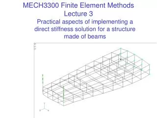
MECH3300 Finite Element Methods Lecture 3 . Practical aspects of implementing a direct stiffness solution for a structure made of beams. Exploiting the sparseness of [K].

E N D
MECH3300 Finite Element Methods Lecture 3 Practical aspects of implementing a direct stiffness solution for a structure made of beams
Exploiting the sparseness of [K] • If degrees of freedom are numbered in the order of the nodes, then if nodes that are connected can be given similar numbers, off-diagonal terms of [K] will correspond to similar row and column numbers. • If this is the case, then [K] is banded. The bandwidth is the maximum number of rows or columns over which non-zero terms occur. • Bandedness can be exploited both when storing [K] and when solving the equations. Large reductions in disk space used and large increases in speed of solution are possible. Non-zero terms zeroes Bandwidth
Exploiting the sparseness of [K] - 2 • Solvers in commercial codes typically either • (a) store and process only terms of [K] within its bandwidth. • (b) use a sparse matrix storage scheme in which only non-zero terms are stored, along with their row and column addresses. • In the former case, several algorithms to renumber nodes are used to find the most compact form of the matrix. The matrix may be stored from the diagonal up to the last nonzero term in each column - this is called a ‘skyline’ form of the matrix. STRAND7 will display the matrix in this form, before and after nodes are renumbered.
Assembly of element matrices in practice Conceptually, element matrices are expanded with rows and columns of zeroes and added. In practice, this amounts to finding the right row and column addresses in the full matrix into which each stiffness term should be placed. To do this a list of the degrees of freedom at each node of an element is first stored for each element, called an element destination vector. 5 2 23 17 6 1 24 18 16 4 3 22 Numbering of rows/columns in [Ke] Numbering of rows/columns of [K] for the same pair of nodes. Element destination vector: [16 17 18 22 23 24] ie row 1 of [Ke] = row 16 of [K] column 5 of [Ke] = column 23 of [K]
Differences between beam elements and a physical beam • One physical beam often needs to divided into several beam elements. • (a) Elements only connect at nodes, • as equations are only written at nodes. If this is one element, it is NOT connected to the vertical one - it needs subdividing. (b) To apply an intermediate load, a beam must be subdivided in order to place a node where the load is applied.
Refinements in modeling beams Moment reactions wL2/12 • Intermediate or distributed loading can be represented by statically equivalent loading at the nodes. The loads to apply are minus the reactions that would occur if the nodes at each end of the element were fixed. wL/2 wL/2 wL2/12 Load w per length wL2/12 Loads applied to model - this causes the correct nodal deflections Force reactions wL/2 L Applied load and fixed-end reactions - this loading causes no nodal deflections. Sum is the applied load only (what we wish to model)
Refinements in modeling beams - 2 • If the centroidal axes of beams do not meet at a joint, one may need to be “offset” - that is, the node must be shifted some distance off the centroidal axis. This can be done in both principal axis directions. Offset of node on the left element.
Refinements to modeling beams - 3 • The default connection is a rigid joint (all members displace and rotate the same at a joint). To create pin joints at particular nodes only, or to create a sliding joint, end-releases are used. • An end-release creates 2 separate degrees of freedom, one on each beam - eg two independent rotations to give a pin joint. • This is useful in modeling a mechanism.
Stresses in beams • Stresses can only be found if the cross-sectional shape of a beam is specified in the data. Often, this is done by giving the positions of the “extreme fibres” - the corners furthest from the centroidal axis. • Stresses consist of axial stress P/A, bending stresses in 2 principal planes, torsional and transverse shear stresses. • A useful combined stress is “total fibre stress” - axial stress plus the stress due to bending in both transverse planes. In the absence of intermediate or distributed loading, the worst stresses are at the nodes. To see stresses, typically a visualisation of the cross-section of a beam is first turned on in a package.
Constraint equations • Extra equations are often added to the set of equations solved, called constraint equations, that relate the motion of different nodes. The user is typically unaware of this, however… • The most common form of constraint equation is one prescribing rigid body behaviour. In STRAND7 this is a “rigid link”. In NASTRAN it is a rigid element, or a multi-point constraint (MPC). • Constraint equations also can be used to apply displacement boundary conditions. In STRAND7, the restraint menu allows a non-zero value to be specified. In NASTRAN, a node must first be fixed and then a load applied to it, with the load redefined as a displacement. ANSYS also regards imposed displacements as loads.
Local axes of a beam The usual convention for local beam axes is as follows. Axis 1 (or local x) is the major principal axis. Axis 2 (or local y) is the minor principal axis and points toward the reference node. Axis 3 (or local z) is along the beam. Note that this means that forces in local axes may have inconsistent signs for different elements, where there is a change in reference node. Axis 2 Reference node in plane of axes 2 and 3 End B End A (1st node chosen when meshing) Axis 3 Axis 1