Download
1 / 19
190 likes | 314 Vues
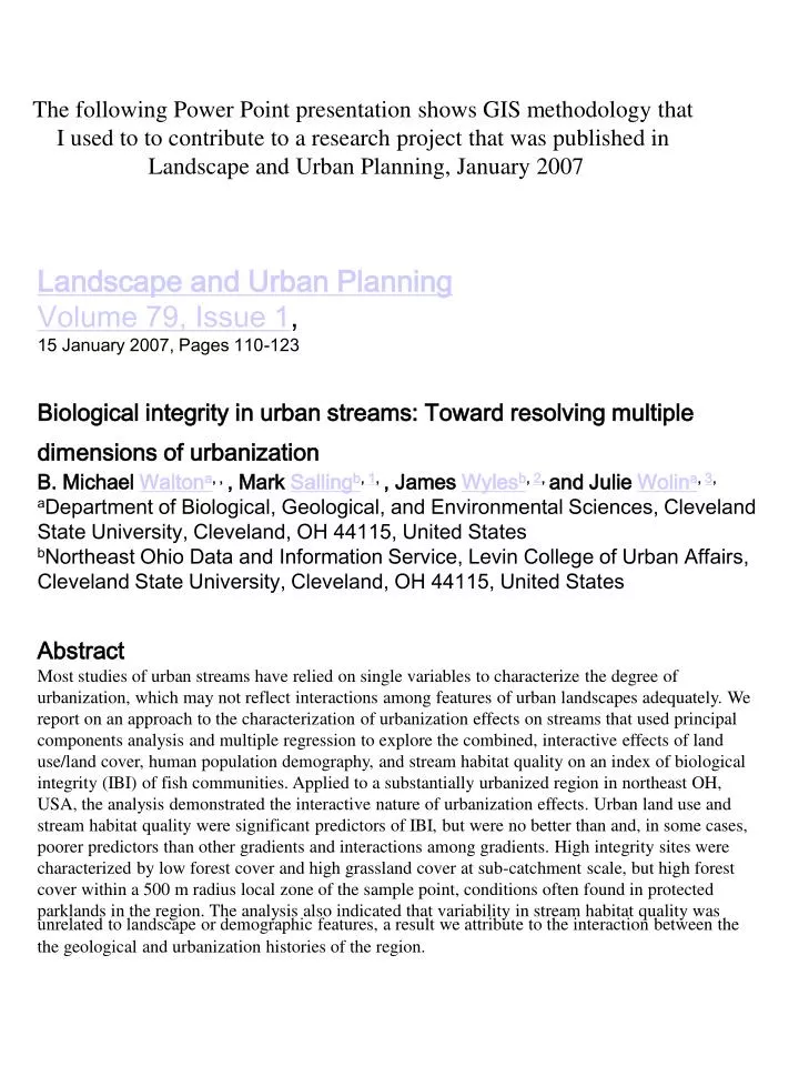
The following Power Point presentation shows GIS methodology that I used to to contribute to a research project that was published in Landscape and Urban Planning, January 2007. Landscape and Urban Planning Volume 79, Issue 1 , 15 January 2007, Pages 110-123

E N D
The following Power Point presentation shows GIS methodology that I used to to contribute to a research project that was published in Landscape and Urban Planning, January 2007 Landscape and Urban PlanningVolume 79, Issue 1, 15 January 2007, Pages 110-123 Biological integrity in urban streams: Toward resolving multiple dimensions of urbanization B. Michael Waltona, , , Mark Sallingb, 1, , James Wylesb, 2, and Julie Wolina, 3, aDepartment of Biological, Geological, and Environmental Sciences, Cleveland State University, Cleveland, OH 44115, United States bNortheast Ohio Data and Information Service, Levin College of Urban Affairs, Cleveland State University, Cleveland, OH 44115, United States Abstract Most studies of urban streams have relied on single variables to characterize the degree of urbanization, which may not reflect interactions among features of urban landscapes adequately. We report on an approach to the characterization of urbanization effects on streams that used principal components analysis and multiple regression to explore the combined, interactive effects of land use/land cover, human population demography, and stream habitat quality on an index of biological integrity (IBI) of fish communities. Applied to a substantially urbanized region in northeast OH, USA, the analysis demonstrated the interactive nature of urbanization effects. Urban land use and stream habitat quality were significant predictors of IBI, but were no better than and, in some cases, poorer predictors than other gradients and interactions among gradients. High integrity sites were characterized by low forest cover and high grassland cover at sub-catchment scale, but high forest cover within a 500 m radius local zone of the sample point, conditions often found in protected parklands in the region. The analysis also indicated that variability in stream habitat quality was unrelated to landscape or demographic features, a result we attribute to the interaction between the the geological and urbanization histories of the region.
GIS Methodology By James C. Wyles
Watershed Selection Criteria based on: • Catchment area size (range- 52 to 130 sq. kilometers) • Catchment portion intersects urbanized area • Sites of “special interest” to regional water management areas • Amount or coverage of available biological data- EPA samples
Project based on Sample Point Catchment Area: Area that drains to a single point until reaching the next upstream sample point catchment or adjoiningsample point catchment • Each catchment polygon represents the drainage area for its corresponding EPA sample site. • Catchment polygons populated with data values that describe land use and selected census variables
Data required to determine catchment areas: • Ohio EPA sample points • Vector stream file- Valley Segment Type rivers (VST) from • National Hydrography Dataset (NHD) of USGS & US EPA • Digital Elevation Model (DEM)- 10 & 30 m cell size from USGS • Flow direction grid • DEM derived streams • Geometric network linking points and streams INPUT OUTPUT
Digital Elevation Model (DEM) Processing • ArcHydro Terrain Processing functions in ESRI ArcGIS • Adjust or enhance DEM using Valley Stream Segment (AGREE) • Fill Sinks • Determine flow direction • Determine flow accumulation • Define stream definition & segmentation • Transform into vector stream drainage Before enhancement
Digital Elevation Model (DEM) Processing • ArcHydro Terrain Processing functions in ESRI ArcGIS • Adjust or enhance DEM using Valley Stream Segment (AGREE) • Fill Sinks • Determine flow direction • Determine flow accumulation • Define stream definition & segmentation • Transform into vector stream drainage After enhancement
Terrain Processing: Drainage Line Processing Vector stream created (DEM Derived Stream)
Terrain Processing: Create catchments • The geometric network consists of 3 data layers- network • junctions, EPA sample points, and the DEM stream. • The flow direction grid and geometric network are used to • delineate the sample point catchment polygon.
Populate Catchments with Data • Land Use (1994 from ODNR) • Clip land use polygons at catchment boundary • Recalculate area in square meters for each land use (Urban, Agricultural/Open Urban Areas, Shrub/Scrub, Wooded, Open Water, Non Forested Wetlands, Barren) • Census (2000 from US Census Bureau) • Clip Census data polygons at catchment boundary • Area proportion field values according to new polygon size • Fields- Year structure built, population,households, & housing units
Create 500 meter Buffer Polygons • within Sample Catchments • why? To determine ifvariations observed in the IBI/ICI data could be • explained by smaller areas of influence • Center of buffer is sample point • Areas outside the 500 m radius or catchment are deleted (clipped) • Recalculate area in square meters for each land use • Area proportion census field values according to new polygon
Create Riparian Buffer Polygons of • 15, 30, 60, 90, 120, &150 meters • from Streams within Sample Catchments • why? To determine ifvariations observed in the IBI/ICI data could be • explained by stream buffers at various distances of influence • Center of buffer is Stream within catchment • Areas outside the buffer zone or catchment are deleted (clipped) • Recalculate area in square meters for each land use • Area proportion Census field values according to new polygon 120 meter Riparian Buffer Example
Determine Downstream Sample Point & Catchment Calculate Downstream Distance Between Sample Points
Create Catchment Aggregation of Urbanization Data by Magnitude • Network trace created to identify all upstream points within the water subshed. • Catchment magnitudes are determined. • Catchment magnitude = 0 means that the data is only aggregated for one specific catchment. • Magnitude = 1 means the data of original catchment and one catchment level upstream • of the current catchment are aggregated. • Catchment magnitude is determined until proceeding upstream to the headwaters. • Land use and Census data are aggregated by the magnitude of the catchment. • River length, the average and sum of stream distances are calculated per magnitude.