Download
1 / 53
1.02k likes | 4.16k Vues
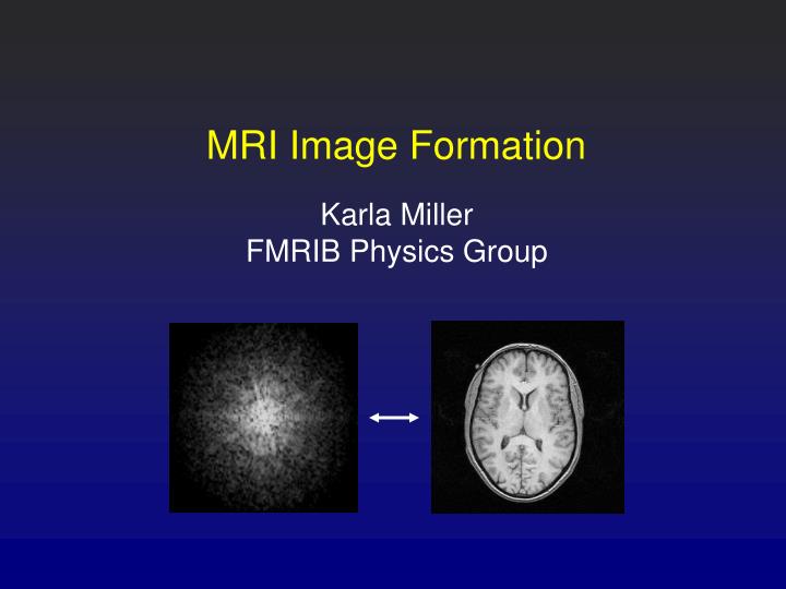
MRI Image Formation. Karla Miller FMRIB Physics Group. Image Formation. Gradients and spatial encoding Sampling k -space Trajectories and acquisition strategies Fast imaging Acquiring multiple slices Image reconstruction and artifacts. field strength. field offset.

E N D
MRI Image Formation Karla Miller FMRIB Physics Group
Image Formation • Gradients and spatial encoding • Sampling k-space • Trajectories and acquisition strategies • Fast imaging • Acquiring multiple slices • Image reconstruction and artifacts
field strength field offset MR imaging is based on precession z y x [courtesy William Overall] Spins precess at the Larmor rate: • = g (B0 + DB)
High field B0 Low field Magnetic Gradients Gradient: Additional magnetic field which varies over space • Gradient adds to B0, so field depends on position • Precessional frequency varies with position! • “Pulse sequence” modulates size of gradient
High field B0 Low field Magnetic Gradients • Spins at each position sing at different frequency • RF coil hears all of the spins at once • Differentiate material at a given position by selectively listening to that frequency Fast precession Slow precession
Simple “imaging” experiment (1D) increasing field
Simple “imaging” experiment (1D) Signal Fourier transform “Image” position Fourier Transform: determines amount of material at a given location by selectively “listening” to the corresponding frequency
y ky 1D Signal 1D “Image” x kx 2DFT 1DFT 2D Signal 2D Image 2D Imaging via 2D Fourier Transform
y ky x kx 2D Fourier Transform 2DFT Measured signal (frequency-, or k-space) Reconstructed image FT can be applied in any number of dimensions MRI: signal acquired in 2D frequency space (k-space) (Usually) reconstruct image with 2DFT
Gradients and image acquisition • Magnetic field gradients encode spatial position in precession frequency • Signal is acquired in the frequency domain (k-space) • To get an image, acquire spatial frequencies along both x and y • Image is recovered from k-space data using a Fourier transform
Image Formation • Gradients and spatial encoding • Sampling k-space • Trajectories and acquisition strategies • Fast imaging • Acquiring multiple slices • Image reconstruction and artifacts
x x x x x x x x x x x x x x x x x x x x x x x x x x x x x x x x x x x x x x x x x x x x x x x x x x x x x x x x x x x x x x x x x x x x x x x x x x x x x x x x x x x x x x x x x x x x x x x x x x x x x x x x x x x x x x x x x x x x x x x x x x x x x x x x x x x x x x x x x x x x x x x FT Sampling k-space Perfect reconstruction of an object would require measurement of all locations in k-space (infinite!) Data is acquired point-by-point in k-space (sampling)
kx ky kx 2 kxmax Sampling k-space • What is the highest frequency we need to sample in k-space (kmax)? • How close should the samples be in k-space (Dk)?
Frequency spectrum What is the maximum frequency we need to measure? Or, what is the maximum k-space value we must sample (kmax)? FT -kmax kmax
Frequency spectrum Higher frequencies make the reconstruction look more like the original object! Large kmax increases resolution (allows us to distinguish smaller features)
2D Extension increasing kmax kymax kxmax kxmax kymax 2 kxmax kmaxdetermines image resolution Large kmaxmeans high resolution !
kx ky kx 2 kxmax Sampling k-space • What is the highest frequency we need to sample in k-space (kmax)? • How close should the samples be in k-space (Dk)?
Nyquist Sampling Theorem A given frequency must be sampled at least twice per cycle in order to reproduce it accurately 1 samp/cyc 2 samp/cyc Upper waveform is resolved! Cannot distinguish between waveforms
increasing field Nyquist Sampling Theorem Insufficient sampling forces us to interpret that both samples are at the same location: aliasing
Aliasing (ghosting): inability to differentiate between 2 frequencies makes them appear to be at same location x x Aliased image Applied FOV max ive frequency max ive frequency
kx ky FOV = 1/kx kx x= 1/(2*kxmax) 2 kxmax k-space relations:FOV and Resolution
kx ky xmax = 1/kx kx 2 kxmax = 1/x 2 kxmax k-space relations:FOV and Resolution k-space and image-space are inversely related: resolution in one domain determines extent in other
k-space Image Full-FOV, high-res Full sampling 2DFT Full-FOV, low-res: blurred Reduce kmax Low-FOV, high-res: may be aliased Increase k
Image Formation • Gradients and spatial encoding • Sampling k-space • Trajectories and acquisition strategies • Fast imaging • Acquiring multiple slices • Image reconstruction and artifacts
Visualizing k-space trajectories kx(t) = Gx(t) dt ky(t) = Gy(t) dt k-space location is proportional to accumulated area under gradient waveforms Gradients move us along a trajectory through k-space !
Raster-scan (2DFT) Acquisition Acquire k-space line-by-line (usually called “2DFT”) Gx causes frequency shift along x: “frequency encode” axis Gy causes phase shift along y: “phase ecode” axis
Echo-planar Imaging (EPI) Acquisition Single-shot (snap-shot): acquire all data at once
SNR Ttotal = N Tread Trajectory considerations • Longer readout = more image artifacts • Single-shot (EPI & spiral) warping or blurring • PR & 2DFT have very short readouts and few artifacts • Cartesian (2DFT, EPI) vs radial (PR, spiral) • 2DFT & EPI = ghosting & warping artifacts • PR & spiral = blurring artifacts • SNR for N shots with time per shot Tread :
Image Formation • Gradients and spatial encoding • Sampling k-space • Trajectories and acquisition strategies • Fast imaging • Acquiring multiple slices • Image reconstruction and artifacts
Partial k-space If object is entirely real, quadrants of k-space contain redundant information 2 1 c+id a+ib aib cid ky 3 4 kx
Partial k-space Idea: just acquire half of k-space and “fill in” missing data Symmetry isn’t perfect, so must get slightly more than half 1 c+id a+ib measured data aib cid missing data ky kx
ky ky kx kx Multiple approaches Acquire half of each frequency encode Reduced phase encode steps
Parallel imaging(SENSE, SMASH, GRAPPA, iPAT, etc) Surface coils Object in 8-channel array Single coil sensitivity Multi-channel coils: Array of RF receive coils Each coil is sensitive to a subset of the object
Parallel imaging(SENSE, SMASH, GRAPPA, iPAT, etc) Surface coils Object in 8-channel array Single coil sensitivity Coil sensitivity to encode additional information Can “leave out” large parts of k-space (more than 1/2!) Similar uses to partial k-space (faster imaging, reduced distortion, etc), but can go farther
Image Formation • Gradients and spatial encoding • Sampling k-space • Trajectories and acquisition strategies • Fast imaging • Acquiring multiple slices • Image reconstruction and artifacts
Slice Selection RF frequency 0 gradient Gz excited slice
t1 t2 t3 t4 t5 t6 2D Multi-slice Imaging excited slice All slices excited and acquired sequentially (separately) Most scans acquired this way (including FMRI, DTI)
excited volume “True” 3D imaging excited volume Repeatedly excite all slices simultaneously, k-space acquisition extended from 2D to 3D Higher SNR than multi-slice, but may take longer Typically used in structural scans
Image Formation • Gradients and spatial encoding • Sampling k-space • Trajectories and acquisition strategies • Fast imaging • Acquiring multiple slices • Image reconstruction and artifacts
Motion Artifacts Motion causes inconsistencies between readouts in multi-shot data (structurals) Usually looks like replication of object edges along phase encode direction PE
Gibbs Ringing (Truncation) Abruptly truncating signal in k-space introduces “ringing” to the image
EPI distortion (warping) field offset image distortion Field map EPI image (uncorrected) Magnetization precesses at a different rate than expected Reconstruction places the signal at the wrong location
EPI unwarping (FUGUE) field map uncorrected corrected Field map tells us where there are problems Estimate distortion from field map and remove it