Download

1 / 53
530 likes | 993 Vues
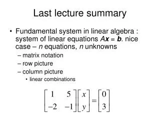
Last lecture summary. Orthogonal matrices. independent basis, orthogonal basis, orthonormal vectors, normalization Put orthonormal vectors into a matrix Generally rectangular matrix – matrix with orhonormal columns Square matrix with orthonormal colums – orthogonal matrix Q

E N D
independent basis, orthogonal basis, orthonormal vectors, normalization • Put orthonormal vectors into a matrix • Generally rectangular matrix – matrix with orhonormal columns • Square matrix with orthonormal colums – orthogonal matrix Q • Matrix A has non-orthogonal columns, A → Q … Gram-Schmidt Orthogonalization • Q-1 = QT
Having Q simplifies many formulas. e. g. • QR decomposition: A = QR
Properties: • Exchange rows/cols of a matrix: reverse sign of det • Equals to 0 if two rows/cols are same. • Det of triangular matrix is a product of diagonal terms. • determinant is a test for invertibility • matrix is invertible if |A| ≠ 0 • matrix is singular if |A| = 0
Action of matrix A on vector x returns the vector parallel (same direction) to vector x. • x … eigenvectors, λ … eigenvalues • spectrum, trace (sum of λ), determinant (product of λ) • λ = 0 … singular matrix • Find eigendecomposition by solving characteristic equation (leading to characteristic polynomial) det(A - λI) = 0 • Find λfirst, then find eigenvectors by Gauss elimination, as the solution of (A - λI)x = 0.
algebraic multiplicity of an eigenvalue • multiplicity of the corresponding root • geometric multiplicity of an eigenvalue • number of linearly independent eigenvectors with that eigenvalue • degenerate, deffective matrix
Diagonalization • Square matrix A …diagonalizable if there exists an invertible matrix P such that P−1AP is a diagonal matrix. • Diagonalization … process of finding a corresponding diagonal matrix. • Diagonalization of square matrix with independent eigenvectors meas its eigendecomposition S-1AS = Λ
Which matrices are diagonalizable (i.e. eigendecomposed)? • all λ’s are different (λ can be zero, the matrix is still diagonalizable. But it is singular.) • if some λ’s are same, I must be careful, I must check the eigenvectors. • If I have repeated eigenvalues, I may or may not have n independent eigenvectors. • If the eigenvectors are independent, than it is diagonalizable (even if I have some repeating eigenvalues). • Diagonalizability is concerned with eigenvectors. (independent) • Invertibility is concerned with eigenvalues. (λ=0)
diagonal matrix • eigenvalues are on the diagonal • eigenvectors are columns with 0 and 1 • triangular matrix • eigenvalues are sitting along the diagonal • symmetric matrix (n x n) • real eigenvalues, real eigenvectors • n independent eigenvectors • they can be chosen such that they are orthonormal (A = QΛQT) • orthogonal matrix • eigenvalues are +1 or -1
Symmetric matrices • eigenvalues are real, eigenvectors are orthogonal (may be chosen to be orthogonal) • Symmetric matrices with all the eigenvalues positive are called positive definite (semidefinite). • A linear system of equations with a positive definite matrix can be efficiently solved using the so-called Cholesky decomposition. • M = LLT = RTR (L – lower triangular, R – upper) • ATA is always symmetric positive definite provided that all columns of A are independent.
Singular Value Decomposition based on excelent video lectures by Gilbert Strang, MIT http://ocw.mit.edu/OcwWeb/Mathematics/18-06Spring-2005/VideoLectures/detail/lecture29.htm Lecture 29
SVD demonstration • we have vectors x and y perpendicular, find such Ax and Ay that are also perpendicular • If found, let’s label x as v1 and y as v2. And Axas u1 and Ayas u2. • If v1 and v2 are orthonormal, u1 and u1 are orthogonal. • But can be normalized – multiplied by numbers σ1 and σ2 • http://ocw.mit.edu/ans7870/18/18.06/javademo/SVD/
So matrix A acts on vector v1 and vector σ1u1 is obtained → Av1 = σ1u1 • And similarly Av2= σ2u2 • Generally, this can be written in a matrix form as AV = UΣ • But realize, that columns of V and U are orthonormal. U and V are orthogonal matrices! • AV = UΣ→ A = UΣV-1→ A = UΣVT
Numbers σ are called singular values. • And A = UΣVT is called singular value decomposition (SVD). • Factors: orthogonal matrix, diagonal matrix, orthogonal matrix – all good matrices! • Σ – singular values (diagonal) • columns of U – left singular vectors (orthogonal) • columns of V – right singular vectors (orthogonal) • Any matrix has SVD! • that’s why we actually need two orthogonal matrices
Dimensions in SVD A: m x n U: m x m V: n x n Σ: m x n
Consider case of square full-rank matrix Am xm. • Look again at Av1= σ1u1 • σ1u1is a linear combination of columns of A. Where lies σ1u1? • In C(A) • And where lies v1? • In C(AT) • In SVD I’m looking for an orthogonal basis in row space of A that gets knocked over into an orthogonal basis in column space of A.
Can I construct an orthogonal basis of C(AT)? • Of course I can, Gram-Schmidt does this. • However, when I take such a basis and multiply it by A, there is no reason why the result should also be orthogonal. • I am looking for the special setup, where A turns orthogonal basis vectors from row space into orthogonal basis in the column space.
basis vectors in row space of A basis vectors in column space of A multiplying factors • In case A is symmetric positive definite, the SVD becomes A = QΛQT. • SVD of positive definite matrix directly reveals its eigendecomposition.
SVD of 2 x 2 nonsingular matrix • U, Σ, V are all of 2 x 2 • If A is real, U and V are also real. • The singular values σ are always real, nonegative, and they are conventionally arranged in descending order on the main diagonal of Σ.
SVD of 2 x 2 singular matrix • SVD is rank revealing factorization. rank(A) is the number of nonzero singular values. • Due to the experimental errors matrices are close to singular – rank deficient • SVD helps in this situation by revaling the intrinsic dimension. Close to zero singular values can then be set equal to zero.
In this example 4 x 4 matrix is generated, with 4th column almost equal to c1 – c2. Then the 4th singular is zeroed, and matrix is reconstructed. Matlab code c1=[1 2 4 8]' c2=[3 6 9 12] c3=[12 16 3 5]' c4 = c1-c2+0.0000001*(rand(4,1)) A = [c1 c2 c3 c4] format long [U,S,V]=svd(A) U1 = U; S1=S; V1 = V; S1(4,4)=0.0 B=U1*S1*V1' A-B norm(A-B) help norm
m x n, m > n (overedetermined system) • with all columns independent A = [c1 c2 c3] [U,S,V]=svd(A) U(1:3,1:3)*S(1:3,1:3)*V' complete this to an orthonormal basis for the whole column space Rm i.e. these vectors come from left null space, which is orthogonal to column space complete this by adding zeros
For the system m ≥ n, there exist a version of SVD, called thin or economy SVD. The zero block from Σ is removed, as well as are corresponding columns from U. Dimensions of thin SVD A: m x n U: m x n V: n x n Σ: n x n these are removed
m x n, n > m (underdetermined system) • with all rows independent A = [c1(1:3) c2(1:3) c3(1:3) [15 12 63]'] [U,S,V]=svd(A) U*S(1:3,1:3)*V(1:3,1:3)' complete this to an orthonormal basis for the whole rowspace Rn i.e. these vectors come from null space, which is orthogonal to row space complete this by adding zeros
Basis of C(AT) Basis of C(A) Basis of N(A) Basis of N(AT) • SVD chooses the right basis for the 4 subspaces • AV=UΣ • v1…vr: orthonormal basis in Rn for C(AT) • vr+1…vn: in Rn for N(A) • u1…ur: in Rm for C(A) • ur+1…um: in Rm for N(AT)
Uniqueness of SVD • non-equal singular values (non-degenerate) • U, V are unique except for the signs in columns • Once you decide signs for U (V), signs for V (U) are given so that A = UΣVT is guaranteed • equal non-zero singular values (degenerate) • not unique • if u1 and u2 correspond to the degenerate σ, also their any normalized linear combination is a left singular vector corresponding to σ • the same is true for right singular vectors
Uniqueness of SVD • zero singular values • Corresponding columns of U and V are added • They form basis of N(AT) or N(A). • They are orthonormal each to other and to the rest of right/left singular vectors. • And are not unique.
How do we find SVD? A = UΣVT • I’ve got two orthogonal matrices and I don't want to find them both at once. • I need some expression so U disappears. • Let’s do ATA (nice positive (semi)definite symmetric). What’s the result? • ATA = VΣTUTUΣVT = VΣ2VT This is actually a diagonalization for positive definite ATA = QΛQT V is found by diagonalizing ATA
How to find U? • Look at diagonalization of AAT, so V disappears. • Or compute • So u’s are eigenvectors of ATA, v’s are eigenvectors of AAT. • And eigenvalues are square roots of σ’s. • They are same for ATA and AAT. • They are unique. • They have arbitrary order. However, they are conventionally sorted in decreasing order (u, v must be reordered accordingly)
Example • Rank is? • two, invertible, nonsingular • I'm going to look for two vectors v1 and v2 in the row space, which of course is what? • R2 • And I'm going to look for u1, u2 in the column space, which is also R2, and I'm going to look for numbers σ1, σ2so that it all comes out right.
SVD example • 1st step – ATA • 2nd step – find its eigenvectors (they’ll b the vs) and eigenvalues (squares of the σ) • eigen can be guessed just by looking • what are eigenvectors and their corresponding eigenvalues? • [1 1]T, λ1 = 32 • [-1 1]T, λ2 = 18 • Actually, I made one mistake, do you see which one? • I didn’t normalize eigenvectors, they should be [1/sqrt(2), 1/sqrt(2)]T …
3rd step – AAT, find the u • What are the eigenvectors? • [1 0]T, [0 1]T It’s diagonal, but just by an accident
SVD expansion • Do you remember column times row picture of matrix multiplication? • If you look at the UΣVTmultiplication as at the column times row problem, then you get the SVD expansion. • This is a sum of rank-one matrices. Each of uiviT is called mode.
This expansion is used in data compression application of SVD. We investigate the spectrum of singular values, and based on it we can decide when to stop the expansion. • This actually means that from Σ we remove singular values from the end, and that we remove coresponding columns from U and V.
SVD image compression load clown colormap('gray') image(X) [U,S,V] = svd(X); plot(diag(S)); size(X,1)*size(X,2) p=1;image(U(:,1:p)*S(1:p,1:p)*V(:,1:p)'); size(U,1)*p+size(V',1)*p To reconstruct Ap, we need to store only (m+n)·p words, compared to m·n needed for storage of the full matrix A. Please note, that if you put p = m (for m<n), then we need m2+m·n, which is much more than m·n. So there is apparently some border at which storing SVD matrices increases the storage needs!
Numerical Linear AlgebraMatrix Decompositions based on excelent video lectures by Gilbert Strang, MIT http://ocw.mit.edu/OcwWeb/Mathematics/18-06Spring-2005/VideoLectures/detail/lecture29.htm Lecture 29
Conditioning and stability • two fundamental issues in numerical analysis • Tell us something about the behavior after introduction of small error. • Conditioning – perturbation behavior of a mathematical problem. • Stability - perturbation behavior of an algorithm.
Conditioning • System’s behavior, it has nothing to do with numerical errors (round off). • Example: Ax = b • well-conditioned - small change in A or b results in a small change in the solution b • ill-conditioned - small change in A or b results in a large change in the solution b • Conditioning is quantified by the condition number, by its coupling with machine epsilon (precission) we can then quantify how many significant digits we can trust in the solution.
well-conditioned system small change in result b ill-conditioned system small change in coefficient matrix A
Stability • Algorithm’s behavior, involves rounding errors etc. • Example: • our computer only has two digits of precision (i.e. only two nonzero numbers are allowed) • we have array of 100 numbers [1.00, 0.01, 0.01, 0.01, …] • and we want to sum them • mathematically exact solution is 1.99
unstable So we take the first number (1.00), then add another (1.01), then another …. (1.10), then another (1.11, however, this can’t be stored in two-dogit precission, so computer rounds down to 1.10), …, so the final result is 1.10 (compare to correct result of 1.99) Or we can sort the array first in ascending order [0.01. 0.01, …, 1.00] and then sum: 0.01, 0.02, 0.03, …0.99, 1.99, 1.99 gets round to 2.00 (compare to correct result of 1.99) stable
Matrix factorizations/decompositions • factorization - decomposition of an object into a product of other objects - factors - which when multiplied together give the original . • matrix factorization – product of some nicer/simpler matrices that retain particular properties of the original matrix A • nicer matrices: orthogonal, diagonal, symmetric, triangular
System of equations Ax = b • System of linear equations • It is solved by Gaussian elimination • Gaussian elimination leads to the LU factorization • U is upper traiangular, L is lower triangular with units on the diagonal
Ax = b … LUx = b, we can say Ux = y, and solve Ly = b and then Ux = y. • Why is it advantageous? • Similarly, Ux = y is solved by backward substitution. • LU factorization is Gauss elimination, so when should I do LU factorization? • If I have more bs, but A does not change. I do LU just once, and then I repeatedly change just RHS (b). forward substitution
LU factorization is used to calculate matrix determinant. • A = LU, det(A) = det(LU) = det(L)det(U) = product of diagonal elements L (one) x product of diagonal elements U • Use of QR factorization for Ax = b • A = QR, QRx = b → Rx = QTb • Compute A = QR • Compute y = QTb • solve Rx = y by back-substitution
However the standard way for Ax = b is Gauss (LU), it requires half of the operations than QR. • LU factorization can also be used for matrix inversion (however, standard way is Gauss-Jacobi), L and U are easier to invert.
Least squares algorithms • ATAx = ATb • Least squares via normal equations: • Cholesky factorization ATA = RTR leads to RTRx = ATb • form ATA and ATb • compute Cholesky ATA = RTR • solve lower triangular system RTw = ATb for w • solve upper triangular system Rx = w for x