Download
1 / 29
290 likes | 467 Vues
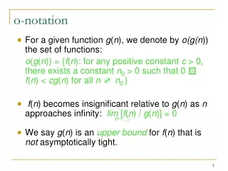
o-notation. For a given function g ( n ), we denote by o (g(n )) the set of functions: o ( g ( n )) = { f ( n ): for any positive constant c > 0, there exists a constant n 0 > 0 such that 0 f ( n ) < cg ( n ) for all n n 0 }

E N D
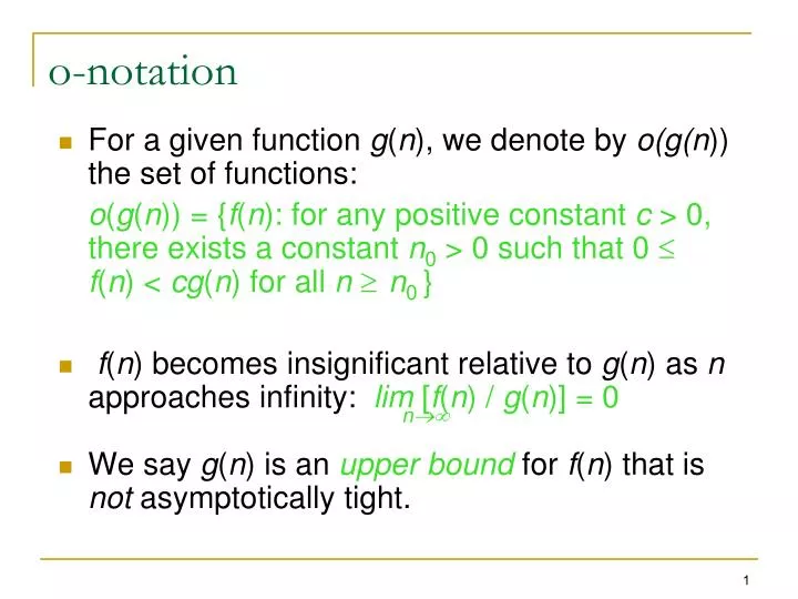
o-notation • For a given function g(n), we denote by o(g(n)) the set of functions: o(g(n)) = {f(n): for any positive constant c > 0, there exists a constant n0 > 0 such that 0 f(n)<cg(n) for all n n0} • f(n) becomes insignificant relative to g(n)as n approaches infinity: lim [f(n) / g(n)] = 0 n • We say g(n) is an upper bound for f(n)that is not asymptotically tight.
O(*) versus o(*) O(g(n)) = {f(n): there exist positive constants c and n0 such that 0 f(n)cg(n), for all n n0}. o(g(n)) = {f(n): for any positive constant c > 0, there exists a constant n0 > 0 such that 0 f(n)<cg(n) for all n n0}. Thus o(f(n)) is a weakened O(f(n)). For example: n2 = O(n2) n2 o(n2) n2 = O(n3) n2 = o(n3)
o-notation • n1.9999 = o(n2) • n2/ lg n = o(n2) • n2o(n2) (just like 2< 2) • n2/1000 o(n2)
w-notation • For a given function g(n), we denote by w(g(n)) the set of functions w(g(n)) = {f(n): for any positive constant c > 0, there exists a constant n0 > 0 such that 0 cg(n)<f(n) for all n n0} • f(n) becomes arbitrarily large relative to g(n)as n approaches infinity: lim [f(n) / g(n)] = n • We say g(n) is a lower bound for f(n)that is not asymptotically tight.
w-notation • n2.0001 = ω(n2) • n2 lg n = ω(n2) • n2ω(n2)
Comparison of Functions f g a b f (n) = O(g(n)) a b f (n) = (g(n)) a b f (n) = (g(n)) a = b f (n) = o(g(n)) a < b f (n) = w (g(n)) a > b
Properties • Transitivity f(n) = (g(n)) & g(n) = (h(n)) f(n) = (h(n)) f(n) = O(g(n)) & g(n) = O(h(n)) f(n) = O(h(n)) f(n) = (g(n)) & g(n) = (h(n)) f(n) = (h(n)) • Symmetry f(n) = (g(n)) if and only if g(n) = (f(n)) • Transpose Symmetry f(n) = O(g(n)) if and only if g(n) = (f(n))
Practical Complexities • Is O(n2) too much time? • Is the algorithm practical? At CPU speed 109 instructions/second
Impractical Complexities At CPU speed 109 instructions/second
Growth Rates of some Functions Polynomial Functions Exponential Functions
Effect of Multiplicative Constant 800 f(n)=n2 600 Run time 400 f(n)=10n 200 0 n 10 20 25
n 2n 1ms x 2n 10 103 0.001 s 20 106 1 s 30 109 16.7 mins 40 1012 11.6 days 50 1015 31.7 years 60 1018 31710 years Exponential Functions • Exponential functions increase rapidly, e.g., 2n will double whenever n is increased by 1.
Floors & Ceilings • For any real number x, we denote the greatest integerless than or equal to x by x • read “the floor of x” • For any real number x, we denote the least integergreater than or equal to x by x • read “the ceiling of x” • For all real x, (example for x=4.2) • x – 1 x x x x + 1 • For any integer n , • n/2 + n/2 = n
Polynomials • Given a positive integer d, a polynomial in n of degree d is a function P(n) of the form • P(n) = • where a0, a1, …, ad are coefficient of the polynomial • ad 0 • A polynomial is asymptotically positive iffad 0 • Also P(n) = (nd)
Exponents • x0 = 1 x1 = x x-1 = 1/x • xa . xb = xa+b • xa / xb = xa-b • (xa)b = (xb)a = xab • xn + xn = 2xn x2n • 2n + 2n = 2.2n = 2n+1
Logarithms (1) • In computer science, all logarithms are to base 2 unless specified otherwise • xa = b iff logx(b) = a • lg(n) = log2(n) • ln(n) = loge(n) • lgk(n) = (lg(n))k • loga(b) = logc(b) / logc(a) ; c 0 • lg(ab) = lg(a) + lg(b) • lg(a/b) = lg(a) - lg(b) • lg(ab) = b . lg(a)
Logarithms (2) • a = blogb(a) • alogb(n) = nlogb(a) • lg (1/a) = - lg(a) • logb(a) = 1/loga(b) • lg(n) n for all n 0 • loga(a) = 1 • lg(1) = 0, lg(2) = 1, lg(1024=210) = 10 • lg(1048576=220) = 20
Summation • Why do we need to know this? We need it for computing the running time of a given algorithm. • Example: Maximum Sub-vector Given an array a[1…n] of numeric values (can be positive, zero and negative) determine the sub-vector a[i…j] (1 i j n) whose sum of elements is maximum over all sub-vectors.
Example: Max Sub-Vectors MaxSubvector(a, n) { maxsum = 0; for i = 1 to n { for j = i to n { sum = 0; for k = i to j { sum += a[k] } maxsum = max(sum, maxsum); } } return maxsum; }
Summation • Constant Series: For a, b 0, • Quadratic Series: For n 0, • Linear-Geometric Series: For n 0,
Proof of Geometric series A Geometric series is one in which the sum approaches a given number as N tends to infinity. Proofs for geometric series are done by cancellation, as demonstrated.
Factorials • n! (“n factorial”) is defined for integers n 0 as • n! = • n! = 1 . 2 .3 … n • n! < nn for n ≥ 2