Download
1 / 65
650 likes | 1.1k Vues
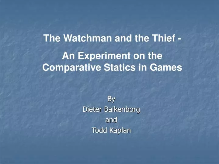
The Watchman and the Thief - An Experiment on the Comparative Statics in Games. By Dieter Balkenborg and Todd Kaplan. Introduction. Mixed strategy: Randomizing between different options Central role of mixed strategy in games

E N D
The Watchman and the Thief - An Experiment on the Comparative Statics in Games By Dieter Balkenborg and Todd Kaplan
Introduction • Mixed strategy: Randomizing between different options • Central role of mixed strategy in games • Mixed strategy as a tool for preventing to be outguessed by the opponent • Bart Simpson in episode 9F16 "Good ol' rock. Nuthin' beats that!“. Lisa: “Poor Bart. He is so predictable.”
von Neumann on game theory Jacob Bronowski recalls in “The Ascent of Man”, BBC, 1973, a conversation with John von Neumann: … I (JB) naturally said to him, since I am an enthusiastic chess player “You mean the theory of games like chess”. “No, no,” he (vN) said. “Chess is not a game. Chess is a well-defined form of computation. You may not be able to work out the answers, but in theory there must be a solution, a right procedure in every position. Now real games,” he said, “are not like that at all. Real life is not like that. Real life consists of bluffing, of little tactics of deception, of asking yourself what is the other man going to think I mean to do. And that is what games are about in my theory.”
Mixed Strategies are a way of remaining unpredictable Penalty Kick: Dive L Dive R 58.3 94.97 Kick L Kick R 92.91 69.92 • “R” = strong side of kicker • Nash prediction for • (Kicker, Goalie)=(41.99L+58.01R, 38.54L+61.46R) • Actual Data =(42.31L+57.69R, 39.98L+60.02R) • Palacios-Huerta (2003), Volij & Palacios-Huerta (2006)
The Watchman and the Thief WATCHMAN Q: How does increase in punishment affect equilibrium behaviour? Watch Rest 4 High Punishment: 6 Home 5 5 WATCHMAN THIEF 6 4 4 Rest Watch Steal 4 4 7 6 ? Home 5 5 THIEF 4 6 ? Steal 1 7 Low Punishment: ? ?
A: Watchman gets more lazy, theft remains as before. WATCHMAN Rest Watch 4 High Punishment: 6 Home 5 5 WATCHMAN THIEF 6 4 4 Rest Watch Steal 4 4 7 6 Home 5 5 THIEF 4 6 Steal 1 7 Low Punishment:
Game Structures: The Watchman and the Thief WATCHMAN Not watching Watching 0 -1 P >0, punishment for the thief. F >0, fine for the watchman. R >0, reward for the watchman. Not stealing 0 0 THIEF -F R Stealing 1 -P
Mixed Strategy Nash Equilibria • Mixed Nash equilibria determined by the condition to make the opponent indifferent • How a player randomizes depends only on payoff of his opponent • Counterintuitive Implications • Relevance for economics: Relevant economic implications (Dasgupta, Stiglitz 1980, Kaplan, Luski, Wettstein 2003) (More firms implies less innovation)
Main design feature • Population design (Nagel, Zamir 2001): • 10 subjects are row players (thieves) • 10 are column players (watchmen) • In each period every thief plays against every watchman and vice versa (10 plays) • Placement random
Questions • Qualitative predictions of theory correct? • “Own Payoff effect” to be expected. Will they be wielded out in market-like matching environment? • Relevance of security strategies?
Literature: • Experiments on normal form games with a unique mixed equilibrium • Atkinson and Suppes (1963) 2x2, 0-sum • O'Neill (1987) 4x4, 0-sum • Malawski (1989) 2x2, 3x3 game • Brown & Rosenthal (1990) 4x4, 0-sum • Rapoport & Boebel (1992) 5x5 • Mookerherjee & Sopher (1994) matching pennies • Bloomfield (1995) 2x2, r. dev, • Ochs (1995) 2x2, compet., r.d., r.m. • Mookerherjee & Sopher (1997) 4x4 games, const sum • Erev & Roth (1998) many data sets • McKelvey, Palfrey & Weber (1999) 2x2 • Fang-Fang Tang (1999, 2001, 2003) 3x3 • Rapoport & Almadoss (2000) investment game
Literature (cont): • Goree, Holt, Palfrey (2000) 2x2 , 0-sum • Bracht (2000) 2x2 , 0-sum • Bracht & Ichimura (2002) 2x2, 0-sum • Binmore, Swierpinski & Proulx 2x2, 3x3, 4x4, 0-sum • Shachat (2002) 4x4, 5x5 games, 0-sum • Shachat & Walker 2x2 games • Rosenthal, Shachat & Walker (2001) 2x2 games, 0-sum • Nagel & Zamir (2000) 2x2 games • Selten &Chmura (2005) 2x2 games • Empirical: • Walker and Wooders (2001) tennis • Ciappori, Levitt, Groseclose (2003) soccer • Palacios-Huerta (2003) soccer • Volij & Palacios-Huerta (2006) soccer
Outline • Experimental Design • Aggregate Results • Own payoff Effect • Quantal Response and Risk Aversion • The learning cycle • Individual Behaviour • Heterogeneity • Movers and Shakers • Conclusions
Experimental Design: • Computerized Experiment at FEELE (the Finance and Economics Experimental Laboratory at Exeter University). • Programmed by Tim Miller in z-tree. • A session lasted approx. 1:30 h, on average a student earned £18. • 120 subjects
Written instructions, summary • Test questions • 2 trial rounds • 50 paid rounds • Questionnaire, payment • No “story” • Either row- or column player throughout • Each player makes 10 decisions per period
Six Sessions: • H1: High penalty • H2: High penalty, row interchanged • H3: High penalty, column interchanged • L4: Low penalty • L5: Low penalty, row interchanged • L6: Low penalty, column interchanged (Data adjusted here)
Screen shot: Row players’ decision screen
Screen shot: Column players’ decision screen
Screen shot: Row players’ “waiting” screen
Screen shot: Row players’ result screen
Screen shot: Column players’ result screen
Results 1, Watchmen (col) • The average proportion of watching (R) is lower in the high-punishment treatments. • The observation is robust over time. • High Punishment: Too close to 50%?
Results 2, Thieves (row) average proportion of stealing (B) • (Own-payoff effect): In the high-penalty sessions the average proportion of stealing is 10-15% below equilibrium while it is close to equilibrium in the other session.
Results 3 • The noise in the aggregate per-period data is large. The data fit roughly in a circle of diameter 0.5. • There is no convergence to equilibrium.
1 0.9 0.8 1-p 0.7 0.6 0.5 0.4 0.3 0.2 0.1 0 0 0.1 0.2 0.3 0.4 0.5 0.6 0.7 0.8 0.9 1 q Session H1
1 0.9 0.8 1-p 0.7 0.6 0.5 0.4 0.3 0.2 0.1 0 0 0.1 0.2 0.3 0.4 0.5 0.6 0.7 0.8 0.9 1 q Session H2
1 0.9 0.8 1-p 0.7 0.6 0.5 0.4 0.3 0.2 0.1 0 0 0.1 0.2 0.3 0.4 0.5 0.6 0.7 0.8 0.9 1 q Session H3
1 0.9 0.8 1-p 0.7 0.6 0.5 0.4 0.3 0.2 0.1 0 0 0.1 0.2 0.3 0.4 0.5 0.6 0.7 0.8 0.9 1 q Session L4
1 0.9 0.8 1-p 0.7 0.6 0.5 0.4 0.3 0.2 0.1 0 0 0.1 0.2 0.3 0.4 0.5 0.6 0.7 0.8 0.9 1 q Session L5
1 0.9 0.8 1-p 0.7 0.6 0.5 0.4 0.3 0.2 0.1 0 0 0.1 0.2 0.3 0.4 0.5 0.6 0.7 0.8 0.9 1 q Session L6
PENALTY HIGH WATCH=.28, STEAL=.42 r=0.405808, =0.177009 • PENALTY=1; (HIGH) • WATCH=.28, STEAL=.42 • r=0.405808, =0.177009 • WATCH=.32, STEAL=.36 • r=0.433568, =0.371299 • WATCH=.34, STEAL=.42 • r=0.106692, =0.406645 • PENALTY=4; (LOW) • WATCH=.57, STEAL=.48 • NO CONVERGENCE. • WATCH=.65, STEAL=.52 • r=0.206081, =0.0929088 • WATCH=.51, STEAL=.52 • r=1.46235, =0.194742
Results 4 Fraction of watching. • The trial rounds matter. • The adjustment seems to happen in the first 5 rounds (including trial rounds).
Results 5 • The ten-period moving averages lie in a circle of radius 0.1. Session 6:
Results 6 • The moving averages data points seem to spin counter-clockwise, although not necessarily around the equilibrium. This is indicated in the following graphs.
Session H1 Direction of movement Equilibrium
Session H2 Direction of movement Equilibrium
Session H3 Direction of movement Equilibrium
Session L4 Direction of movement Equilibrium
Session L5 Direction of movement Equilibrium
Direction of movement Equilibrium Session L6
Test 1 • We run a OLS regression on the moving average data using a linear difference equation as the model. • Does the matrix describe a rotation counter-clockwise?
Session H1 Graphical Analysis: Graph exhibiting the DE fitted to the original MA data.The movements are always anticlockwise and converge. Direction of movement Equilibrium
Session H2 Graphical Analysis: Graph exhibiting the DE fitted to the original MA data.The movements are always anticlockwise and converge. Direction of movement Equilibrium
Session L3 Graphical Analysis: Graph exhibiting the DE fitted to the original MA data.The movements are always anticlockwise and converge. Direction of movement Equilibrium