Download

1 / 25
250 likes | 254 Vues
Learn about analyzing algorithms for running time, memory requirements, and more. Explore asymptotic performance and understand Insertion Sort's correctness, properties, and complexities. Discover worst, average, and best-case scenarios in algorithm analysis.

E N D
Analysis of Algorithms Coming up • Asymptotic performance, Insertion Sort • A formal introduction to asymptotic notation (Chap 2.1-2.2, Chap 3.1)
Asymptotic performance In analysis of algorithms, we care most about asymptotic performance “How does the algorithm behave as the problem size gets very large?” • Running time • Memory/storage requirements • Bandwidth/power requirements/logic gates/etc.
4.32 * 10-6sec 5.32 * 10-6sec 5.91 * 10-6sec 4.47 * 10-6sec 6.32 * 10-6sec 7.75 * 10-6sec 20 * 10-6sec 40 * 10-6sec 60 * 10-6sec 86 * 10-6sec 213 * 10-6sec 354 * 10-6sec 400 * 10-6sec 1600 * 10-6sec 3600 * 10-6sec 0.16 sec 2.56 sec 12.96 sec Asymptotic performance Assume: an algorithm can solve a problem of size n in f(n) microseconds (10-6 seconds).
f(n) 90000 log2n 80000 Sqrt n 70000 n 60000 microseconds nlog2n 50000 n2 40000 30000 n4 20000 2n 10000 n n! 0 1 3 5 7 9 13 15 17 19 11 Asymptotic performance Assume: an algorithm can solve a problem of size n in f(n) microseconds (10-6 seconds).
Input Size Time and space complexity is generally a function of the input size E.g., sorting, multiplication How we characterize input size depends: • Sorting: number of input items • Multiplication: total number of bits • Graph algorithms: number of nodes & edges
1 … j j+1..n Currently sorted part Currently unsorted part Insertion Sort To sort A[1..n] in place: • Steps: • Pick element A[j] • Move A[j-1..1] to the right until proper position for A[j] is found.
Correctness of Insertion Sort To prove Insertion Sort is correct, we state the loop invariant: “At start of each iteration of the for loop, A[1..j-1] consists of the elements originally in A[1..j-1] but in sorted order.” We observe 3 properties: Initialization: It is true prior to the first iteration of the loop Maintenance: If it is true before an iteration, it remains true before next iteration. Termination: When the loop terminates, the invariant gives a useful property that helps show the algorithm is correct. Can you state these properties for Insertion Sort?
Correctness of Insertion Sort loop invariant “At start of each iteration of the for loop, A[1..j-1] consists of the elements originally in A[1..j-1] but in sorted order.” Initialization Before the first iteration, j=2. => A[1 .. j-1] contains only A[1]. => Loop invariant holds prior to the first iteration. Maintenance The outer loop moves A[j-1],A[j-2],A[j-3] .. to the right until the proper position for A[j] is founded. Then A[j] is inserted. => if the loop invariant is true before an iteration, it remains true before next iteration. Termination The outer loop ends with j=n+1. Substituting n+1 for j in the loop invariant, we get “A[1..n] consists of the n sorted elements.”
Analyzing Insertion Sort Cost c1 c2 0 c4 c5 c6 c7 c8 times n n-1 n-1 n-1 j=2..n tj j=2..n (tj-1) j=2..n (tj-1) n-1 tj = no. of times that line 5 is executed, for each j. The running time T(n) = c1*n+c2*(n-1)+c4*(n-1)+c5*(j=2..n tj)+c6*(j=2..n (tj-1))+c7*(j=2..n (tj-1))+c8*(n-1)
Analyzing Insertion Sort T(n) = c1*n+c2*(n-1)+c4*(n-1)+c5*(j=2..n tj)+ c6*(j=2..n (tj-1))+c7*(j=2..n (tj-1))+c8*(n-1) Worse case: Reverse sorted inner loop body executed for all previous elements. tj=j. T(n) = c1*n+c2*(n-1)+c4*(n-1)+c5*(j=2..n j)+ c6*(j=2..n (j-1))+c7*(j=2..n (j-1))+c8*(n-1) T(n) = c1*n+c2*(n-1)+c4*(n-1)+c5*(j=2..n j)+ c6*(j=2..n (j-1))+c7*(j=2..n (j-1))+c8*(n-1) T(n) = An2+Bn+C Noting: j=2..n j = __________ j=2..n (j-1) = _______
Analyzing Insertion Sort T(n)=c1*n+c2*(n-1)+c4*(n-1)+c5*(j=2..n tj)+c6*(j=2..n (tj-1))+c7*(j=2..n (tj-1))+c8*(n-1) Worst case Reverse sorted => inner loop body executed for all previous elements. So, tj=j. => T(n) is quadratic: T(n)=An2+Bn+C Average case Half elements in A[1..j-1] are less than A[j]. So, tj = j/2 => T(n) is also quadratic: T(n)=An2+Bn+C Best case Already sorted => inner loop body never executed. So, tj=1. => T(n) is linear: T(n)=An+B
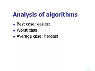
Kinds of Analysis (Usually) Worst case: T(n) = max time on any input of size n • Knowing it gives us a guarantee about the upper bound. • In some cases, worst case occurs fairly often • Average case is often as bad as worst case. (Sometimes) Average case: T(n) = average time over all inputs of size n (Rarely) Best case: Cheat with slow algorithm that works fast on some input. Good only for showing bad lower bound.
Random-Access Machine Analysis is performed with respect to a computational model We usually use a generic uniprocessor random-access machine (RAM) • All memory equally expensive to access • No concurrent operations • All reasonable instructions take unit time (Except, of course, function calls) Constant word size
Order of Growth • Ignore machine-dependent constants • Look at growth of T(n) as n -> • Drop low-order terms, Ignore leading constants Eg. worse case of insertion sort, T(n) = An2+Bn+C T(n) = An2+Bn+C Order of Growth = n2 “T(n) is in (n2)” • For convenience, we usually say “T(n) is (n2)” and “T(n) = (n2)” • An algorithm is more efficient if its worst-case running time has a lower order of growth. (n2) is a set of functions that relates to n2 in some way. (We’ll define later)
Asymptotic Notations 3 major notations for describing algorithm complexities: Asymptotic Tight Bound: Intuitively like “=” Asymptotic Upper Bound: Intuitively like “” Asymptotic Lower Bound: Intuitively like “” Other notations: o, Intuitively like “<” and “>” Eg., Insertion Sort’s worse case running time is (n2). Insertion Sort’s best case running time is (n). Insertion Sort’s running time is (n). Insertion Sort’s running time is O(n2). .. running time is in(n2).
Asymptotic Notations Very often the algorithm complexity can be observed directly from simple algorithms: The levels of nested loops. • O(n2) • (n)
cg(n) f(n) n0 f(n) is O(g(n)) f(n) cg(n) n0 f(n) is (g(n)) c2g(n) f(n) c1g(n) n0 f(n) is (g(n)) Definitions of O, , and O(g(n)) = { f(n): there exist positive constants c and n0 such that 0 f(n) cg(n) for all n n0 } (g(n)) = { f(n): there exist positive constants c and n0 such that 0 cg(n) f(n) for all n n0 } (g(n)) = { f(n): there exist positive constants c1, c2, n0 such that 0 c1g(n) f(n) c2g(n) for all n n0 } (g(n)) <=> O(g(n)) and (g(n))
Example According to the formal definition of , prove that 0.5n2 - 3n = (n2) To do so, we must determine positive constants c1, c2, n0 such that c1n2 0.5n2-3n c2n2, for all n n0. Dividing by n2 yields: c1 0.5 - 3/n c2. • c1 0.5-3/n holds for any value of n7 by choosing c11/14 • 0.5-3/n c2 holds for any value n 1 by choosing c2 0.5 Hence by choosing c1=1/14, c2=0.5, and n0=7, we can verify that 0.5n2 - 3n = (n2).
Example (cont’d) • We have shown that 0.5n2 - 3n = (n2). Similar prove can be applied to show An2+Bn+C = (n2) and An+B = (n). • For insertion sort: Worse case running time: T(n) = An2+Bn+C => T(n) = (n2) Average case running time: T(n) = An2+Bn+C => T(n) = (n2) Best case running time: T(n) = An+B => T(n) = (n) • Recall that, informally, the () term can be obtained by observing the highest order term and drop the leading constant.
Example According to the formal definition of O, prove that 6n3O(n2) Prove by contradiction: Suppose c, n0 exist such that 6n3 cn2, for all n n0. => n c2/6, which is impossible for arbitrarily large n, since c is a constant. => 6n3 cn2 is not correct => 6n3O(n2)
Points to Note • We can write 2n2+3n+1 = 2n2+ (n). f(n) = n2 + O(n) means f(n) = n2 + h(n) for some h(n) O(n) • O-notation is an upper-bound notation. It makes no sense to say f(n) is at least O(n). Why? • It is also correct to write n2=O(n3), and n2= (n). Proof?
Analysis of Algorithms Summary • Algorithm, input, output, instance, “Correct Algorithm” (recall Introduction) • Asymptotic Performance, Input Size • Insertion Sort • Proof: Insertion Sort is correct (Loop Invariant + 3 properties) • Analysis of Insertion Sort, Worse/Average/Best case • Order of Growth • Asymptotic Notations