Download
1 / 19
200 likes | 228 Vues
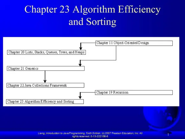
Algorithm Efficiency. Yih-Kuen Tsay Dept. of Information Management National Taiwan University Based on [ Carrano and Henry 2013] With help from Chien Chin Chen. A Larger Picture. Efficiency is just one aspect in evaluating a solution/program. What is a good computer program?

E N D
Algorithm Efficiency Yih-Kuen Tsay Dept. of Information Management National Taiwan University Based on [Carrano and Henry 2013] With help from Chien Chin Chen
A Larger Picture • Efficiency is just one aspect in evaluating a solution/program. • What is a good computer program? • Aspects to consider: • Correctness (consequence of errors) • Efficiency: time and memory required to execute • Ease of use • Effort required to develop, maintain, modify, and expand DS 2016: Algorithm Efficiency
Programs vs. Algorithms • The underlying algorithm (including the objects and how they interact) has the most significant impact on the efficiency of a program. • Three fundamental problems with comparing programs instead of algorithms: • How are the algorithms coded? • Different implementations, different run times • What computer should you use? • Faster on one computer, but slower on another • What data should the programs use? • Different data sets, different run times DS 2016: Algorithm Efficiency
Measuring Algorithm Efficiency (1/4) • Analysis of algorithms: • Provides tools for contrasting the efficiency of different algorithms. • Time and space efficiency • Concerns with significant differences in efficiency, not reductions in computing costs due to clever coding tricks • We will focus on time efficiency. DS 2016: Algorithm Efficiency
Measuring Algorithm Efficiency (2/4) • Algorithm analysis should be independent of : • Specific implementations • Computers • Data • How? • Counting the number of significant operations in a particular solution. • Significant operations are those which consume most computing time. DS 2016: Algorithm Efficiency
Measuring Algorithm Efficiency (3/4) • We have compared solutions by looking at the number of operations that each solution requires. • An algorithm’s execution time is related to the number of operations it requires. • This is usually expressed in terms of the number nof items the algorithm must process. DS 2016: Algorithm Efficiency
Measuring Algorithm Efficiency (4/4) • Example: traversal of a linked list of n nodes. • n + 1 assignments, n + 1 comparisons, n writes. • Suppose each assignment, comparison, and write takes respectively a, c, and w time units. • The traversal takes (n + 1)×(a + c) + n×w time units. • Example: the Towers of Hanoi with n disks. • 2n - 1 moves. • If each move takes the same time m, then the solution takes (2n - 1 )×m time units. 1 assignment Node<ItemType>* curPtr= headPtr; while(curPtr!= nullptr) { cout << curPtr->getItem() << endl; curPtr= curPtr->getNext(); } // end while n+1 comparisons n writes n assignments DS 2016: Algorithm Efficiency
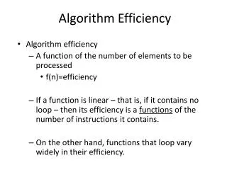
Algorithm Growth Rates (1/3) • An algorithm’s time requirements can be measured as a function of the problem size (instance characteristic). • Number of nodes in a linked list • Size of an array • Number of items in a stack • Number of disks in the Towers of Hanoi problem • Algorithm efficiency is typically a concern for large problems only. DS 2016: Algorithm Efficiency
Algorithm Growth Rates (2/3) Source: FIGURE 10-1 in [Carrano and Henry 2013]. DS 2016: Algorithm Efficiency
Algorithm Growth Rates (3/3) • An algorithm’s growth rate: • How quickly the algorithm’s time requirement grows as a function of the problem size. • Algorithm A requires time proportional to n2. • Algorithm B requires time proportional to n. • Algorithm B is faster than algorithm A. • n2 and n above are growth-rate functions. • Will study a mathematical notation for specifying an algorithm’s order in terms of the size of the problem. • Algorithm A is O(n2) - order n2. • Algorithm B is O(n) - order n. DS 2016: Algorithm Efficiency
Analysis and Big O Notation (1/5) • Definition of the order of an algorithm: Algorithm A is order f(n)– denoted O(f(n))– if constants k and n0 exist such that A requires no more than k × f(n) time units to solve a problem of size n ≥ n0. • The function f(n) is called the algorithm’s growth-rate function. • Because of the capital O to denote order, it is called the Big O Notation. • Examples: • Traversal of a linked list is O(n) • The Towers of Hanoi is O(2n) DS 2016: Algorithm Efficiency
Analysis and Big O Notation (2/5) • O(1) < O(log2n) < O(n) < O(n × log2n) < O(n2) < O(n3) < O(2n). constant logarithmic linear n log n quadratic cubic exponential Source: FIGURE 10-3(a) in [Carrano and Henry 2013]. DS 2016: Algorithm Efficiency
Analysis and Big O Notation (3/5) Source: FIGURE 10-3(b) in [Carrano and Henry 2013]. DS 2016: Algorithm Efficiency
Analysis and Big O Notation (4/5) • Properties of growth-rate functions: • O(n3 + 3n) is O(n3): ignorelow-order terms. • O(5 f(n)) = O(f(n)): ignore a multiplicative constant in the high-order term. • O(f(n)) + O(g(n)) = O(f(n) + g(n)). • O(f(n)) × O(g(n)) = O(f(n) ×g(n)). DS 2016: Algorithm Efficiency
Analysis and Big O Notation (5/5) • An algorithm may require different times to solve different problems of the same size. • Best-case analysis • A determination of the minimum amount of time that an algorithm requires to solve problems of size n. • Worst-case analysis • A determination of the maximum amount of time that an algorithm requires to solve problems of size n. • Easier to calculate and more common. • Average-case analysis • A determination of the average amount of time that an algorithm requires to solve problems of size n. • Usually hard to calculate. DS 2016: Algorithm Efficiency
Keeping Your Perspective (1/2) • Only significant differences in efficiency are interesting. • Frequency of operations: • When choosing an ADT’s implementation, consider how frequently particular ADT operations occur in a given application. • However, some seldom-used but critical operations must be efficient. • E.g., an air traffic control system. DS 2016: Algorithm Efficiency
Keeping Your Perspective (2/2) • If the problem size is always small, you can probably ignore an algorithm’s efficiency. • Order-of-magnitude analysis focuses on large problems. • Weigh the trade-offs between an algorithm’s time requirements and its memory requirements. • Compare algorithms for both style and efficiency. DS 2016: Algorithm Efficiency
Efficiency of Searching Algorithms (1/2) • Sequential search • Strategy: • Look at each item in the data collection in turn. • Stop when the desired item is found, or the end of the data is reached. • Efficiency • Worst case: O(n) DS 2016: Algorithm Efficiency
Efficiency of Searching Algorithms (2/2) • Binary search of a sorted array • Strategy: • Repeatedly divide the array in halves. • Determine which half could contain the item, and discard the other half. • Efficiency • Worst case: • For large arrays, the binary search has an enormous advantage over a sequential search. • At most 20 comparisons to search an array of one million items. • Note, however, there is an overhead of maintaining the array in sorted order. O(log2n) DS 2016: Algorithm Efficiency