Download

1 / 6
70 likes | 238 Vues
Root Locus Design. 7.6 Root Locus Design Example. Consider rigid satellite control system. motor. compensator. R(s). +. K. –. j. +. K V. – j. The RL is along the j axis, then the system will always oscillate regardless the value of K.

E N D
7.6 Root Locus Design Example. Consider rigid satellite control system motor compensator R(s) + K – j + KV –j The RL is along the j axis, then the system will always oscillate regardless the value of K. To obtain an acceptable design the following system will be employed motor compensator R(s) A(s) + K – R(s) The open loop-function is now:
7.6 Root Locus Design And the RL is The rate feedback changes the gain to KKv and add a zero at s = - 1/Kv . The system is seen to be stable for all K and Kv positive. Since there are 2 parameters K and Kv, the poles theoretically can be placed anywhere in the s plane. However it must be remembered that the physical system always has limitation. The rate feedback is actually a PD compensation with TF j –j A problem with PD compensator is that its gain increases with frequency. If high frequency noise presents another compensator (phase lead) can be used to limit the high frequency gain.
j 2 poles –j PHASE LEAD DESIGN The TF of 1st order phase lead compensator is given by The angle criteria is (all zero angles) – (all pole angles) = r consider the RL of the uncompensated is Where |z0| < |p0|, and Kc, z0, and p0are to be determined to satisfy the design criteria. First before we present the design procedure we consider the CE of compensated system Adding the lead compensation the root locus will shift the RL to the left. Suppose S1 is on the RL then θz – θp- 2θ1=-180 j θ1 θz θp The product of KKc can be considered as single gain parameter p0 z0 –j 2 poles
Analytical Phase Lead Design ao can be chosen arbitrarily, a1 and a2is computed using (7.53) from the reference book For this procedure it is convenient to express lead compensator as The object of the design is to choose a0,a1, and b1 suchthat given s1 That is we design the compensator places the pole at s1. Here we have 4 unknowns with only 2 equations (magnitude and angle). We can choose K=1 leaving 3 unknown. ao can be chosen arbitrarily
j 2 poles –j Analytical Phase Lead Design The angle criteria is (all zero angles) – (all pole angles) = r consider the RL of the uncompensated is a0,a1, and b1 Adding the lead compensation the root locus will shift the RL to the left. Suppose S1 is on the RL then θz – θp- 2θ1=-180 That is we design the compensator places the pole at s1. Here we have 4 unknowns with only 2 equations (magnitude and angle). We can choose K=1 leaving 3 unknown j θ1 θz θp p0 z0 –j 2 poles