Download
1 / 9
90 likes | 442 Vues
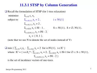
11.3.1 STSP by Column Generation. Recall the formulation of STSP (for 1-tree relaxation) minimize eE c e x e subject to e({ i }) x e = 2 , i N{ 1} e({1}) x e = 2 , eE (S) x e |S| - 1 , S N{ 1}, S , N{ 1}, e E (N{ 1}) x e = |N| - 2.

E N D
11.3.1 STSP by Column Generation • Recall the formulation of STSP (for 1-tree relaxation) minimize eEcexe subject to e({i})xe = 2 , i N\{1} e({1})xe = 2 , eE(S)xe |S| - 1 , S N\{1}, S , N\{1}, eE(N\{1})xe = |N| - 2. xe { 0, 1 }. (note that we use N to denote the set of nodes instead of V) • min { eEcexe : e(i)xe = 2 for iN\{1}, xX1 } where X1 = { xZ+m : e(1)xe = 2, eE(S)xe |S|-1 for S N\{1}, eE(N\{1})xe = |N| - 2 } is the set of incidence vectors of one-trees.
STSP: min { eEcexe : e(i)xe = 2 for iN\{1}, xX1 } where X1 = { xZ+m : e(1)xe = 2, eE(S)xe |S|-1 for S N\{1}, eE(N\{1})xe = |N| - 2 } is the set of incidence vectors of one-trees. • Write xe = t : eE(t) t , t {0, 1}, where Gt = (N, Et) is the tth one-tree. e(i)xe = e(i) t : eE(t) t = t ditt = 2 (dit is degree of node i in the one-tree Gt.) (In matrix notation, we have Ax = 2, where A is the node-edge incidence matrix (for edges E(N\{1})). x = T, where each column of T is incidence vector of a one-tree. AT = 2 (each column of AT is ATt ) )
min t=1T1 (cxt)t (DW) t=1T1ditt = 2, for i N\{1} t=1T1 t = 1 B|T1| • LP relaxation is: min t=1T1 (cxt)t (LPM) t=1T1ditt = 2, for i N\{1} t=1T1 t = 1 R+T1 • Note that the convexity constraintt=1T1 t = 1 (t=1T12t = 2) may be regarded as d1t= 2 for node 1. • Subproblem: 1= min{eE(ce- ui- uj)xe - : xX1} (e=(i, j)E, i, jN\{1}) ( cxt - iN\{1}ditui - = cxt - iN\{1}ui e(i)xet - = eE (ce - ui - uj)xet - )
11.3.2 Strength of the LP Master • Prop 11.1: zLPM = max { k=1Kckxk : k=1KAkxk = b, xk conv(Xk) for k = 1, … , K } Pf) LPM is obtained from IP by substituting xk = t=1Tkxk, tk, t, t=1Tkk, t = 1, k, t 0 for t = 1, … , Tk . This is equivalent to substituting xk conv(Xk). • Prop 11.1 implies that the previous column generation approach for STSP provides the same bound as Lagrangean dual. • Let wLD be the value of the Lagrangian dual when the joint constraint k=1KAkxk = b are dualized. Let zCUT be the optimal value obtained when cutting planes are added to the LP relaxation of IP using exact separation algorithm for each of conv(Xk) for k = 1, … , K. Then Thm 11.2:zLPM= wLD = zCUT
Hence column generation approach (if it can be used for the problem) usually provides strong bounds. • It uses the dual variables obtained from LP relaxation as guides compared to simple rule of subgradient method for Lagrangian dual. (Some more discussions on this later.) • Generated columns can be kept for overall optimization. (compare to Lagrangian dual) • Consider column generation algorithm for generalized assignment problem and its merits compared to Lagrangian dual and cutting plane algorithms. (See Savelsbergh, A Branch and Price Algorithm for the Generalized Assignment Problem, Operations Research, 1997, Vol 45, No 6, p831-841)
11.4 IP Column Generation for 0-1 IP • Branch-and-price algorithm How to branch after column generation? • (IP) z = max { k=1Kckxk : k=1KAkxk = b, Dkxk dk for k = 1, … , K, xk for k = 1, … , K}, reformulation z = max k=1K t=1Tk ( ckxk, t ) k, t (IPM) k=1K t=1Tk ( Akxk, t ) k, t = b t=1Tkk, t = 1 for k = 1, … ,K k, t {0, 1} for t = 1, … , Tk and k = 1, … , K if and only if is integer
If LP relaxation of IPM has fractional solution, two choices to branch : (1) on x variable, (2) on variable. (Following are general schemes. Particular implementation may vary and/or even very difficult.) • Consider branch on x variables If fractional in LP optimal, there is some and j such that the corresponding 0-1 variable xj has LP value that is fractional. Split the set S of all feasible solutions into S0 = S { x: xj = 0} and S1 = S { x: xj = 1} Now as xjk = t=1Tkk, txjk, t {0, 1}, xjk = {0, 1} implies that xjk, t = for all k, t with k, t > 0
Hence the Master Problem at node Si = S { x: xj = i} for i = 0, 1 is z(Si) = max k t ( ckxk, t ) k, t + (IPM(Si)) k t ( Akxk, t ) k, t + = b t k, t = 1 for k = 1 k, t {0, 1} for t = 1, … , Tk , k = 1, … , K The columns for k = are affected. Column generation for subproblem and i = 0, 1 (Si) = max { (c - A) x - : x X , xj = i }
Branch on variables If k, t fractional, fix it to 0 and 1 respectively. If fixed to 1, no problem in column generation. ( usually implemented by setting the lower and upper bound on k, t as 1) If fixed to 0 ( set upper bound of k, t to 0), we need a scheme to prevent the generation of the same column again in the column generation procedure. • Also the branching may partition the set of feasible solutions unbalanced.