Download
1 / 24
250 likes | 463 Vues
Electron & Hole Statistics in Semiconductors A “Short Course”. BW, Ch. 6 & S. Ch 3. The following discussion assumes a basic knowledge of elementary statistical physics . We know that The electronic energy levels in the bands ,

E N D
Electron & Hole Statistics in SemiconductorsA “Short Course”. BW, Ch. 6 & S. Ch 3
The following discussion assumes a basic knowledge of elementary statistical physics. • We know that The electronic energy levels in the bands, which are solutions to the Schrödinger Equation in the periodic crystal, are actually NOT continuous, but are really discrete. We have always treated them as continuous, because there are so many levels& they are so very closely spaced.
Even though we normally treat these levels as if they were continuous, for the next discussion, lets treat them as discrete for a while. • Assume that there are Nenergy levels (N >>>1): ε1, ε2, ε3, … εN-1, εN with degeneracies: g1, g2,…,gN • Results fromquantum statistical physics: Electrons have the following Fundamental Properties: They are indistinguishable particles For statistical purposes, they are Fermions, Spin s = ½
So, electrons are indistinguishable Fermions, with Spin s = ½ • This means that they obey the Pauli Exclusion Principle: That is, when doing statistics (counting) for the occupied states: There can be at most, one e- occupying a given quantum state(including spin) • Consider the band state labeled nk (energy Enk, & wavefunction nk). It can hold, at most, 2 e- : 1 e- with spin “up” ( ) + 1 e- with spin “down” ( ). So, energy level Enk can have up to 2 e-: or 1 e- : or1 e- : , or 0 e- : __
Fermi-Dirac Distribution • Statistical Mechanics Results for Electrons: Consider a system of n e-, with N Single e- Levels (ε1, ε2, ε3, … εN-1, εN ) with degeneracies (g1, g2,…, gN) at absolute temperature T: • In every statistical physics book, it is proven that the probability that energy level εj, with degeneracy gj, is occupied is: (<nj/gj ) ≡ (exp[(εj - εF)/kBT] +1)-1 (< ≡ ensemble average, kB ≡ Boltzmann’s constant) Physical Interpretation <nj = average number of e- in energy level εjat temperature T εF≡ Fermi Energy(or Fermi Level, discussed next)
Define: The Fermi-Dirac Distribution Function (or Fermi distribution) f(ε) ≡ (exp[(ε - εF)/kBT] +1)-1 • The probability of occupation of level j is (<nj/gj ) ≡ f(ε)
Now, lets look at theFermi Functionin more detail. f(ε) ≡ (exp[(ε - εF)/kBT] +1)-1 • Physical InterpretationofεF≡Fermi Energy: εF≡The energy of the highest occupied level at T = 0. • Consider the limitT 0. It’s easily shown that: f(ε) 1, ε < εF f(ε) 0, ε > εF and, for all T f(ε) = ½, ε = εF
The Fermi Function: • f(ε) ≡ (exp[(ε - εF)/kBT] +1)-1 • LimitT 0: f(ε) 1, ε < εF • f(ε) 0, ε > εF • for all T f(ε) = ½, ε = εF • What is the order of magnitude of εF? Any solid state physics text discusses a simple calculation of εF. • Typically, it is found, in temperature units that εF 104 K. • Compare with room temperature (T 300K): • kBT (1/40) eV 0.025 eV • So, obviouslywe always haveεF >> kBT
Fermi-Dirac Distribution NOTE! Levels within ~ kBT of εF(in the “tail”, where it differs from a step function) are the ONLY ones which enter conduction (transport) processes! Within that tail, f(ε) ≡ exp[-(ε - εF)/kBT] ≡ Maxwell-Boltzmann distribution
“Free Electrons” in Metals at 0 K • Simple calculations of the Fermi Energy EF& related properties for a Free Electron Gas. Fermi Energy EFEnergy of the highest occupied state Fermi VelocityvF Velocity of an electron with energy EF Fermi Temperature TF Velocity of electron with energy EF Fermi NumberkFWave number of an electron with energy EF Fermi WavelengthλFWavelength of an electron with energy EF ηeElectron Density in the material
Sketch of a typical experiment. A sample of metal is “sandwiched” between two larger sized samples of an insulator or semiconductor. Vacuum Level Metal Band Edge F EF EF Fermi Energy F Work Function Energy
Using typical numbers in the formulas for several metals & calculating gives the table below:
f k T B 1 T = 0 K Vacuum Occupation Probability, Level Increasing T 0 E F F Work Function, Electron Energy, E Effect of Temperature Fermi-Dirac Distribution
Number and Energy Densities Number density: Energy density: Density of StatesNumber of electron states available between energies E &E+dE. For 3D spherical bands only, it’s easily shown that:
T Dependences of e- & e+ Concentrations n concentration (cm-3) of e-, p concentration (cm-3) of e+ • Using earlier results & making the Maxwell-Boltzmann approximation to the Fermi Function for energies near EF, it can be shown that np= CT3 exp[- Eg/(kBT)] (C = material dependent constant) • In a pure material:n = p ni(np = ni2) ni“Intrinsic carrier concentration”. So, ni= C1/2T3/2exp[- Eg/(2kBT)] At T = 300K Si : Eg= 1.2 eV, ni=~ 1.5 x 1010 cm-3 Ge : Eg= 0.67 eV, ni=~ 3.0 x 1013 cm-3
Intrinsic Concentration vs. T Measurements/Predictions Note the different scales on the right & left figures!
Doped Materials: Materials with Impurities! As already discussed, these are more interesting & useful! • Consider an idealized carbon (diamond) lattice (we could do the following for any Group IV material). C : (Group IV) valence = 4 • Replace one C with a phosphorous. P : (Group V) valence = 5 4 e- go to the 4 bonds 5th e- ~ is “almost free” to move in the lattice (goes to the conduction band; is weakly bound). • P donates 1 e-to the material P is a DONOR (D) impurity
Doped Materials We’ve shown earlier how to calculate this! • The 5th e- is really not free, but is loosely bound with energy ΔED<< Eg The 5th e- moves when an E field is applied! It becomes a conduction e- • Let: Dany donor, DX neutral donor D+ ionized donor (e-to the conduction band) • Consider the chemical “reaction”: e- + D+ DX + ΔED As T increases, this “reaction” goes to the left. But, it works both directions
Consider very high T All donors are ionized n = NDconcentration of donor atoms (constant, independent of T) • It is still true that np = ni2 = CT3 exp[- Eg/(kBT)] p = (CT3/ND)exp[- Eg/(kBT)] “Minority carrier concentration” • All donors are ionized The minority carrier concentration is Tdependent. • At still higher T, n >>> ND, n ~ ni The range of T where n = ND the “Extrinsic” Conduction region.
n vs. 1/T Almost no ionized donors & no intrinsic carriers lllll High T Low T
Again, consider an idealized C (diamond) lattice. (or any Group IV material). C : (Group IV) valence = 4 • Replace one C with a boron. B : (Group III) valence = 3 • B needs one e- to bond to 4 neighbors. • B can capture e- from a C e+ moves to C (a mobile hole is created) • B accepts 1 e- from the material B is an ACCEPTOR (A) impurity
The hole e+ is really not free. It is loosely bound by energy ΔEA<< Eg Δ EA = Energy released when B captures e- e+ moves when an E field is applied! • NA Acceptor Concentration • Let A any acceptor, AX neutral acceptor A- ionized acceptor (e+ in the valence band) • Chemical “reaction”: e++A- AX + ΔEA As T increases, this “reaction” goes to the left. But, it works both directions Just switch n & p in the previous discussion!
Terminology “Compensated Material” ND = NA “n-Type Material” ND > NA (n dominates p: n > p) “p-Type Material” NA > ND (p dominates n:p > n)