Download
1 / 144
1.45k likes | 1.65k Vues
Aerodynamic Drag Prediction Using Unstructured Mesh Solvers. Dimitri J. Mavriplis National Institute of Aerospace Hampton, Virginia, USA. Overview. Introduction Physical model fidelity Grid resolution and discretization issues

E N D
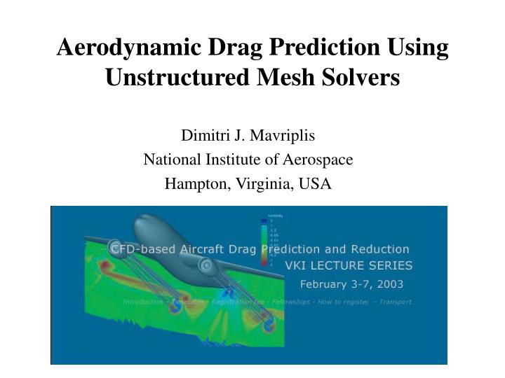
Aerodynamic Drag Prediction Using Unstructured Mesh Solvers Dimitri J. Mavriplis National Institute of Aerospace Hampton, Virginia, USA VKI Lecture Series, February 3-7, 2003
Overview • Introduction • Physical model fidelity • Grid resolution and discretization issues • Designing an efficient unstructured mesh solver for computational aerodynamics • Drag prediction using unstructured mesh solvers • Conclusions and future work VKI Lecture Series, February 3-7, 2003
Overview • Introduction • Importance of Drag Prediction • Suitability of Unstructured Mesh Approach • Physical model fidelity • Inviscid Flow Analysis • Coupled Inviscid-Viscous Methods • Large-Eddy Simulations (LES and DES) VKI Lecture Series, February 3-7, 2003
Overview • Grid resolution and discretization issues • Choice of discretization and effect of dissipation • Cell centered vs. vertex based • Effect of discretization variations on drag prediction • Grid resolution requirements • Choice of element type • Grid resolution issues • Grid convergence VKI Lecture Series, February 3-7, 2003
Overview • Designing an efficient unstructured mesh solver for computational aerodynamics • Discretization • Solution Methodologies • Efficient Hardware Usage VKI Lecture Series, February 3-7, 2003
Overview • Drag prediction using unstructured mesh solvers • Wing-body cruise drag • Incremental effects: engine installation drag • High-lift flows • Conclusions and Future Work VKI Lecture Series, February 3-7, 2003
Introduction • Importance of Drag Prediction • Cruise: fuel burn, range, etc… • High-lift: Mechanical simplicity, noise • High accuracy requirements • Absolute or incremental: 1 drag count • Specialized computational methods • Wide range of scales • Thin boundary layers • Transition VKI Lecture Series, February 3-7, 2003
Introduction • Issues centric to unstructured mesh approach • Advantages and drawbacks over other approaches • Accuracy, efficiency • State-of-the art in aerodynamic predictions • De-emphasize non-method specific issues • Validation/ verification • Drag integration VKI Lecture Series, February 3-7, 2003
CFD Perspective on Meshing Technology • Sophisticated Multiblock Structured Grid Techniques for Complex Geometries Engine Nacelle Multiblock Grid by commercial software TrueGrid.
CFD Perspective on Meshing Technology • Sophisticated Overlapping Structured Grid Techniques for Complex Geometries Overlapping grid system on space shuttle (Slotnick, Kandula and Buning 1994)
Unstructured Grid Alternative • Connectivity stored explicitly • Single Homogeneous Data Structure VKI Lecture Series, February 3-7, 2003
Characteristics of Both Approaches • Structured Grids • Logically rectangular • Support dimensional splitting algorithms • Banded matrices • Blocked or overlapped for complex geometries • Unstructured grids • Lists of cell connectivity, graphs (edge,vertices) • Alternate discretizations/solution strategies • Sparse Matrices • Complex Geometries, Adaptive Meshing • More Efficient Parallelization VKI Lecture Series, February 3-7, 2003
Unstructured Meshes for Aerodynamics • Computational aerodynamics rooted in structured methods • High accuracy and efficiency requirements • Unstructured mesh methods 2 to 4 times more costly • Mitigated by extra structured grid overhead • Block structured • Overset mesh • Parallelization • Accuracy considerations • Validation studies, experience • Unstructured mesh solvers potentially more efficient than structured mesh alternatives with equivalent accuracy VKI Lecture Series, February 3-7, 2003
Physical Model Fidelity • State-of-the-art in drag prediction: RANS • Entire suite of tools available to designer • Useful to examine capabilities of other tools • Lower fidelity – lower costs • Numerous rapid tradeoff studies • Higher fidelity – higher costs • Fewer detailed analyses • Situate RANS tools within this suite VKI Lecture Series, February 3-7, 2003
Physical Model Requirements(Unstructured Mesh Methods) VKI Lecture Series, February 3-7, 2003
Unstructured Mesh Euler Solvers • Inviscid flow unstructured mesh solvers well established – robust • No viscous effects • No turbulence/transition modeling • Isotropic meshes • Good commercial isoptropic mesh generators • Good convergence properties VKI Lecture Series, February 3-7, 2003
Example: Euler Solution of DLR-F4 Wing-body Configuration • 235,000 vertex mesh • (ICEMCFD tetra) • Fully tetrahedral mesh • Convergence in 50 cycles • (multigrid) • 3 minutes on 8 Pentiums • 50 times faster than RANS VKI Lecture Series, February 3-7, 2003
Example: Euler Solution of DLR-F4 Wing-body Configuration • 235,000 vertex mesh • (ICEMCFD tetra) • Fully tetrahedral mesh • Convergence in 50 cycles • (multigrid) • 3 minutes on 8 Pentiums • 50 times faster than RANS VKI Lecture Series, February 3-7, 2003
Example: Euler Solution of DLR-F4 Wing-body Configuration • 235,000 vertex mesh • (ICEMCFD tetra) • Fully tetrahedral mesh • Convergence in 50 cycles • (multigrid) • 3 minutes on 8 Pentiums • 50 times faster than RANS • 1.65 million vertices VKI Lecture Series, February 3-7, 2003
Euler vs. RANS Solution Euler Solution (235,000 pts) RANS Solution (1.65M pts) • 235,000 vertex mesh • (ICEMCFD tetra) • Fully tetrahedral mesh • Convergence in 50 cycles • (multigrid) • 3 minutes on 8 Pentiums • 50 times faster than RANS VKI Lecture Series, February 3-7, 2003
Euler vs. RANS Solution • Exclusion of viscous effects • Boundary layer displacement • Incorrect shock location • Incorrect shock strength • Supercritical wing sensitive to viscous effects • Euler solution not useful for transonic cruise drag prediction VKI Lecture Series, February 3-7, 2003
Coupled Euler-Boundary Layer Approach • Incorporate viscous effects to first order • Boundary layer displacement thickness • More accurate shock strength/location • Retain efficiency of Euler solution approach • Isotropic tetrahedral meshes • Fast, robust convergence VKI Lecture Series, February 3-7, 2003
Coupled Euler-Boundary Layer Approach • Stripwise 2-dimensional boundary layer • 18 stations on wing alone • Interpolate from unstructured surface mesh • Transpiration condition for simulated BL displacement thickness VKI Lecture Series, February 3-7, 2003
Euler vs. RANS Solution Euler Solution (235,000 pts) RANS Solution (1.65M pts) • 235,000 vertex mesh • (ICEMCFD tetra) • Fully tetrahedral mesh • Convergence in 50 cycles • (multigrid) • 3 minutes on 8 Pentiums • 50 times faster than RANS VKI Lecture Series, February 3-7, 2003
Euler-IBL vs. RANS Solution Euler-IBL Sol. (235,000 pts) RANS Solution (1.65M pts) • 235,000 vertex mesh • (ICEMCFD tetra) • Fully tetrahedral mesh • Convergence in 50 cycles • (multigrid) • 3 minutes on 8 Pentiums • 50 times faster than RANS VKI Lecture Series, February 3-7, 2003
Coupled Euler-Boundary Layer Approach VKI Lecture Series, February 3-7, 2003
Coupled Euler-Boundary-Layer Approach • Vastly improved over Euler alone • Correct shock strength, location • Accurate lift • Reasonable drag • More sophisticated coupling possible • 25 times faster than RANS • Neglibible IBL compute time • Convergence dominated by coupling • Parameter studies • Design optimization VKI Lecture Series, February 3-7, 2003
LES and DES Methods • RANS failures for separated flows • Good cruise design involves minimal separation • Off design, high-lift • LES or DES as alternative to turbulence modeling inadequacies • LES: compute all scales down to inertial range • Based on universality of inertial range • DES: hybrid LES/RANS (near wall) • Reduced cost VKI Lecture Series, February 3-7, 2003
LES and DES: Notable Successes • European LESFOIL program • Marie and Sagaut: LES about airfoil near stall • DES for massively separated aerodynamic flows • Strelets 2001, Forsythe 2000, 2001, 2003 • Two to ? Orders of magnitude more expensive than RANS • Predictive ability for accurate drag not established • RANS methods state-of-art for foreseeable future VKI Lecture Series, February 3-7, 2003
Grid Resolution and Discretization Issues • Choice of discretization and effect of dissipation (intricately linked) • Cells versus points • Discretization formulations • Grid resolution requirements • Choice of element type • Grid resolution issues • Grid convergence VKI Lecture Series, February 3-7, 2003
Cell Centered vs Vertex-Based • Tetrahedral Mesh contains 5 to 6 times more cells than vertices • Hexahedral meshes contain same number of cells and vertices (excluding boundary effects) • Prismatic meshes: cells = 2X vertices • Tetrahedral cells : 4 neighbors • Vertices: 20 to 30 neighbors on average VKI Lecture Series, February 3-7, 2003
Cell Centered vs Vertex-Based • On given mesh: • Cell centered discretization: Higher accuracy • Vertex discretization: Lower cost • Equivalent Accuracy-Cost Comparisons Difficult • Often based on equivalent numbers of surface unknowns (2:1 for tet meshes) • Levy (1999) • Yields advantage for vertex-discretization VKI Lecture Series, February 3-7, 2003
Cell Centered vs Vertex-Based • Both approaches have advantages/drawbacks • Methods require substantially different grid resolutions for similar accuracy • Factor 2 to 4 possible in grid requirements • Important for CFD practitioner to understand these implications VKI Lecture Series, February 3-7, 2003
Example: DLR-F4 Wing-body (AIAA Drag Prediction Workshop) VKI Lecture Series, February 3-7, 2003
Illustrative Example: DLR-F4 • NSU3D: vertex-based discretization • Grid : 48K boundary pts, 1.65M pts (9.6M cells) • USM3D: cell-centered discretization • Grid : 50K boundary cells, 2.4M cells (414K pts) • Uses wall functions • NSU3D: on cell centered type grid • Grid: 46K boundary cells, 2.7M cells (470K pts) VKI Lecture Series, February 3-7, 2003
Cell versus Vertex Discretizations • Similar Lift for both codes on cell-centered grid • Baseline NSU3D (finer vertex grid) has lower lift VKI Lecture Series, February 3-7, 2003
Cell versus Vertex Discretizations • Pressure drag • Wall treatment discrepancies • NSU3D : cell centered grid • High drag, (10 to 20 counts) • Grid too coarse for NSU3D • Inexpensive computation • USM3D on cell-centered grid closer to NSU3D on vertex grid Concentrate exclusively on Vertex-Discretizations VKI Lecture Series, February 3-7, 2003
Grid Resolution and Discretization Issues • Choice of discretization and effect of dissipation (intricately linked) • Cells versus points • Discretization formulations • Grid resolution requirements • Choice of element type • Grid resolution issues • Grid convergence VKI Lecture Series, February 3-7, 2003
Discretization • Governing Equations: Reynolds Averaged Navier-Stokes Equations • Conservation of Mass, Momentum and Energy • Single Equation turbulence model (Spalart-Allmaras) • Convection-Diffusion – Production • Vertex-Based Discretization • 2nd order upwind finite-volume scheme • 6 variables per grid point • Flow equations fully coupled (5x5) • Turbulence equation uncoupled VKI Lecture Series, February 3-7, 2003
Spatial Discretization • Mixed Element Meshes • Tetrahedra, Prisms, Pyramids, Hexahedra • Control Volume Based on Median Duals • Fluxes based on edges • Single edge-based data-structure represents all element types Fik = F(uL) + F(uR) + T |L| T-1 (uL –uR) - Upwind discretization - Matrix artificial dissipation VKI Lecture Series, February 3-7, 2003
Upwind Discretization • First order scheme • Second order scheme • Gradients evaluated at vertices by Least-Squares • Limit Gradients for Strong Shock Capturing
Matrix Artificial Dissipation • First order scheme • Second order scheme • By analogy with upwind scheme: • Blending of 1st and 2nd order schemes for strong shock capturing VKI Lecture Series, February 3-7, 2003
Entropy Fix L matrix: diagonal with eigenvalues: u, u, u, u+c, u-c • Robustness issues related to vanishing eigenvalues • Limit smallest eigenvalues as fraction of largest eigenvalue: |u| + c • u = sign(u) * max(|u|, d(|u|+c)) • u+c = sign(u+c) * max(|u+c|, d(|u|+c)) • u – c = sign(u -c) * max(|u-c|, d(|u|+c)) VKI Lecture Series, February 3-7, 2003
Entropy Fix • u = sign(u) * max(|u|, d(|u|+c)) • u+c = sign(u+c) * max(|u+c|, d(|u|+c)) • u – c = sign(u -c) * max(|u-c|, d(|u|+c)) d = 0.1 : typical value for enhanced robustness d = 1.0 : Scalar dissipation - L becomes scaled identity matrix • T |L| T-1 becomes scalar quantity • Simplified (lower cost) dissipation operator • Applicable to upwind and art. dissipation schemes VKI Lecture Series, February 3-7, 2003
Discretization Formulations • Examine effect of discretization type and parameter variations on drag prediction • Effect on drag polars for DLR-F4: • Matrix artificial dissipation • Dissipation levels • Entropy fix • Low order blending • Upwind schemes • Gradient reconstruction • Entropy fix • Limiters VKI Lecture Series, February 3-7, 2003
Effect of Artificial Dissipation Level • Increased accuracy through lower dissipation coef. • Potential loss of robustness
Effect of Entropy Fix for Artificial Dissipation Scheme • Insensitive to small values of d=0.1, 0.2 • High drag values for large d and scalar scheme
Effect of Artificial Dissipation VKI Lecture Series, February 3-7, 2003
Effect of Low-Order Dissipation Blending for Shock Capturing • Lift and drag relatively insensitive • Generally not recommended for transonics
Comparison of Discretization Formulation (Art. Dissip vs. Grad. Rec.) • Least squares approach slightly more diffusive • Extremely sensitive to entropy fix value