Insertion Sort

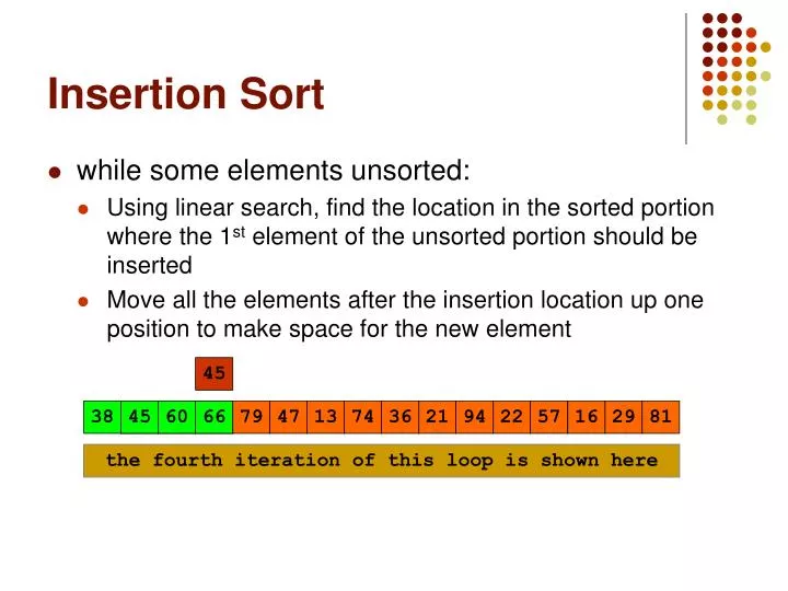
1. Insertion Sort • while some elements unsorted: • Using linear search, find the location in the sorted portion where the 1st element of the unsorted portion should be inserted • Move all the elements after the insertion location up one position to make space for the new element 45 38 60 45 60 66 45 66 79 47 13 74 36 21 94 22 57 16 29 81 the fourth iteration of this loop is shown here

2. An insertion sort partitions the array into two regions

3. An insertion sort of an array of five integers

4. Insertion Sort Algorithm publicvoid insertionSort(Comparable[] arr) { for (int i = 1; i < arr.length; ++i) { Comparable temp = arr[i]; int pos = i; // Shuffle up all sorted items > arr[i] while (pos > 0 && arr[pos-1].compareTo(temp) > 0) { arr[pos] = arr[pos–1]; pos--; } // end while // Insert the current item arr[pos] = temp; } }

5. outer loop outer times inner loop inner times Insertion Sort Analysis publicvoid insertionSort(Comparable[] arr) { for (int i = 1; i < arr.length; ++i) { Comparable temp = arr[i]; int pos = i; // Shuffle up all sorted items > arr[i] while (pos > 0 && arr[pos-1].compareTo(temp) > 0) { arr[pos] = arr[pos–1]; pos--; } // end while // Insert the current item arr[pos] = temp; } }

6. Insertion Sort: Number of Comparisons Remark: we only count comparisons of elements in the array.

7. Insertion Sort: Cost Function • 1 operation to initialize the outer loop • The outer loop is evaluated n-1 times • 5 instructions (including outer loop comparison and increment) • Total cost of the outer loop: 5(n-1) • How many times the inner loop is evaluated is affected by the state of the array to be sorted • Best case: the array is already completely sorted so no “shifting” of array elements is required. • We only test the condition of the inner loop once (2 operations = 1 comparison + 1 element comparison), and the body is never executed • Requires 2(n-1) operations.

8. Insertion Sort: Cost Function • Worst case: the array is sorted in reverse order (so each item has to be moved to the front of the array) • In the i-th iteration of the outer loop, the inner loop will perform 4i+1 operations • Therefore, the total cost of the inner loop will be 2n(n-1)+n-1 • Time cost: • Best case: 7(n-1) • Worst case: 5(n-1)+2n(n-1)+n-1 • What about the number of moves? • Best case: 2(n-1) moves • Worst case: 2(n-1)+n(n-1)/2

9. Insertion Sort: Average Case • Is it closer to the best case (n comparisons)? • The worst case (n * (n-1) / 2) comparisons? • It turns out that when random data is sorted, insertion sort is usually closer to the worst case • Around n * (n-1) / 4 comparisons • Calculating the average number of comparisons more exactly would require us to state assumptions about what the “average” input data set looked like • This would, for example, necessitate discussion of how items were distributed over the array • Exact calculation of the number of operations required to perform even simple algorithms can be challenging(for instance, assume that each initial order of elements has the same probability to occur)

10. Bubble Sort • Simplest sorting algorithm • Idea: • 1. Set flag = false • 2. Traverse the array and compare pairs of two consecutive elements • 1.1 If E1  E2 -> OK (do nothing) • 1.2 If E1 > E2 then Swap(E1, E2) and set flag = true • 3. repeat 1. and 2. while flag=true.

11. Bubble Sort • 1 23 2 56 9 8 10 100 • 1 2 23 56 9 8 10 100 • 1 2 23 9 56 8 10 100 • 1 2 23 9 8 56 10 100 • 1 2 23 9 8 10 56 100 ---- finish the first traversal ---- • 1 2 23 9 8 10 56 100 • 1 2 9 23 8 10 56 100 • 1 2 9 8 23 10 56 100 • 1 2 9 8 10 23 56 100 ---- finish the second traversal ---- …

12. Bubble Sort publicvoid bubbleSort (Comparable[] arr) { boolean isSorted = false; while (!isSorted) { isSorted = true; for (i = 0; i<arr.length-1; i++) if (arr[i].compareTo(arr[i+1]) > 0) { Comparable tmp = arr[i]; arr[i] = arr[i+1]; arr[i+1] = tmp; isSorted = false; } } }

13. Bubble Sort: analysis • After the first traversal (iteration of the main loop) – the maximum element is moved to its place (the end of array) • After the i-th traversal – largest i elements are in their places • Time cost, number of comparisons, number of moves -> Assignment 4

14. O Notation

15. O-notation Introduction • Exact counting of operations is often difficult (and tedious), even for simple algorithms • Often, exact counts are not useful due to other factors, e.g. the language/machine used, or the implementation of the algorithm (different types of operations do not take the same time anyway) • O-notation is a mathematical language for evaluating the running-time (and memory usage) of algorithms

16. Growth Rate of an Algorithm • We often want to compare the performance of algorithms • When doing so we generally want to know how they perform when the problem size (n) is large • Since cost functions are complex, and may be difficult to compute, we approximate them using O notation

17. Example of a Cost Function • Cost Function: tA(n) = n2 + 20n + 100 • Which term dominates? • It depends on the size of n • n = 2, tA(n) = 4 + 40 + 100 • The constant, 100, is the dominating term • n = 10, tA(n) = 100 + 200 + 100 • 20n is the dominating term • n = 100, tA(n) = 10,000 + 2,000 + 100 • n2 is the dominating term • n = 1000, tA(n) = 1,000,000 + 20,000 + 100 • n2 is the dominating term

18. Big O Notation • O notation approximates the cost function of an algorithm • The approximation is usually good enough, especially when considering the efficiency of algorithm as n gets very large • Allows us to estimate rate of function growth • Instead of computing the entire cost function we only need to count the number of times that an algorithm executes its barometer instruction(s) • The instruction that is executed the most number of times in an algorithm (the highest order term)

19. Big O Notation • Given functions tA(n) and g(n), we can say that the efficiency of an algorithm is of order g(n) if there are positive constants c and m such that • tA(n) ·c.g(n) for all n ¸ m • we write • tA(n) is O(g(n)) and we say that • tA(n) is of order g(n) • e.g. if an algorithm’s running time is 3n + 12 then the algorithm is O(n). If c is 3 and m is 12 then: • 4 * n 3n + 12 for all n 12

20. In English… • The cost function of an algorithm A, tA(n), can be approximated by another, simpler, function g(n) which is also a function with only 1 variable, the data size n. • The function g(n) is selected such that it represents an upper bound on the efficiency of the algorithm A (i.e. an upper bound on the value of tA(n)). • This is expressed using the big-O notation: O(g(n)). • For example, if we consider the time efficiency of algorithm A then “tA(n) is O(g(n))” would mean that • A cannot take more “time” than O(g(n)) to execute or that(more than c.g(n) for some constant c) • the cost function tA(n) grows at most as fast as g(n)

21. The general idea is … • when using Big-O notation, rather than giving a precise figure of the cost function using a specific data size n • express the behaviour of the algorithm as its data size n grows very large • so ignore • lower order terms and • constants

22. O Notation Examples • All these expressions are O(n): • n, 3n, 61n + 5, 22n – 5, … • All these expressions are O(n2): • n2, 9 n2, 18 n2+ 4n – 53, … • All these expressions are O(n log n): • n(log n), 5n(log 99n), 18 + (4n – 2)(log (5n + 3)), …