Download
1 / 12
120 likes | 434 Vues
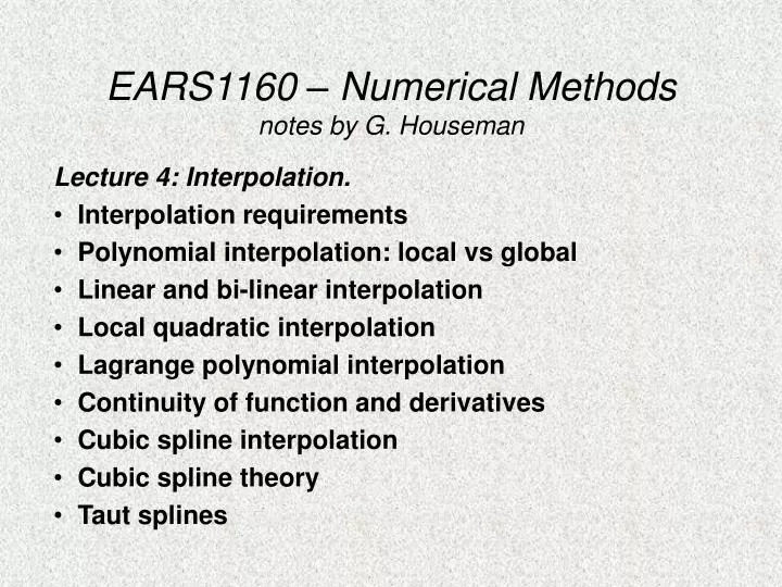
EARS1160 – Numerical Methods notes by G. Houseman. Lecture 4: Interpolation. Interpolation requirements Polynomial interpolation: local vs global Linear and bi-linear interpolation Local quadratic interpolation Lagrange polynomial interpolation Continuity of function and derivatives

E N D
EARS1160 – Numerical Methodsnotes by G. Houseman Lecture 4: Interpolation. • Interpolation requirements • Polynomial interpolation: local vs global • Linear and bi-linear interpolation • Local quadratic interpolation • Lagrange polynomial interpolation • Continuity of function and derivatives • Cubic spline interpolation • Cubic spline theory • Taut splines
f(x) x Dx Interpolation of Discrete Functions Suppose we know the function values at a set of points, e.g. measurement points, how do we find the value of the function at other intermediate (e.g. regularly spaced) points? Ideally we would like to obtain estimates for interpolated points that are consistent with the idea of first (and probably second) derivatives of the interpolated function being continuous. We would also like to be able to extend the method to 2 or more dimensions: f(x,y) or f(x,y,z)
Polynomial Interpolation Example: Magnetic or gravity measurements may be collected at approximately constant spacing along a road or roads. Estimate the interpolated values on a set of regularly spaced points, for display and further processing. Most interpolation methods are based on fitting a polynomial to the data points, and using that polynomial to provide function values at arbitrary points. Global methods attempt to fit a single function to all of the data points. A polynomial of order N-1 may be fit to N data points. Accuracy can be a problem with these methods because they may show large minima and maxima between the points. In general they are not recommended. Local interpolation methods attempt to fit low order polynomials to small subsets of the data. These methods are preferred because they are conceptually simple and they are local, i.e. values of the interpolation function are only influenced by the nearby measurements.
Linear Interpolation The linear interpolation method simply divides the line into segments defined by pairs of adjacent data points. If Then If we write the function in this form, you can simply verify that (i) it is linear in x, and (ii) it gives the required values at the segment end points xk and xk+1. Difficulties with linear interpolation: (i) The slope of the function is discontinuous at all sample points. Higher derivatives are unavailable (ii) Maxima and minima that fall between sample points are poorly represented.
Bi-Linear Interpolation In 2-dimensions the linear interpolation method may be extended for data points that fall approximately on a grid. If, for the point (x, y), and Then This function is linear in x (if y is fixed) or vice versa, but note the presence of a term in xy - which allows us to fit a simple surface to 4 points. A true linear function (representing a plane in 3D) could fit at most 3 points. This method does not necessarily require that the points fall on a regular grid, and may be extended to higher dimensions if necessary.
Local Quadratic Interpolation To improve on linear interpolation, we might consider using local quadratic functions. The quadratic function has 3 unknown coefficients, so two sample points don't provide enough information to constrain the 3 unknowns. If we use 3 adjacent points, we can exactly fit a parabola which covers 2 sampling intervals: Disadvantages: (i) gradient of the function is still discontinuous at every second grid point (ii) odd-numbered points are treated differently from even-numbered points
Polynomial Interpolation formula The equation given above for quadratic interpolation can be generalised to a polynomial of any order: This is the Lagrange polynomial interpolation formula. You can verify by substitution that PN(xj) = f(xj) for each sample point. You will use the routine POLINT from Numerical Recipes (Press et al., 1992) in the next practical exercise. POLINT implements the Lagrange formula using Neville's algorithm which builds the polynomial coefficients recursively.
Continuity A function is continuous if there are no sudden steps in its value as we move along the independent variable. Continuity is usually an essential requirement of an interpolation function. With linear interpolation, sudden changes in slope of the interpolated function are observed at each sample point. A plot of the derivative of the interpolated function looks like a staircase: flat between sample points, then stepping up or down at each sample point. The second derivative is undefined at these points. It is often useful to have continuous first and second derivatives for an interpolated function, since we may want to evaluate these quantities. If 1st derivative is continuous, then discontinuous 2nd derivative is less obvious - it implies a step-like change in curvature of the interpolated function. We refer to C0, C1, and C2 continuity, to indicate continuity of the function, its gradient, and its curvature, respectively.
Cubic Spline Interpolation With local cubic interpolation we can obtain C2 continuity without the stability and accuracy problems associated with the Lagrange Polynomials. A cubic polynomial has 4 coefficients. If we require that the polynomial fits the points at xj and xj+1, then two of the coefficients are specified. If we also require continuity of 1st and 2nd derivatives with the cubic function on the adjoining segments, then we have enough constraints to uniquely define all the coefficients for all the cubic polynomial segments. The resulting function is called a Cubic Spline. The spline functions may be quickly calculated, are accurate and stable, and now are widely used for interpolation in many different applications. We have not yet specified the behaviour of first and second derivatives at the end points of the sample range. There is some choice possible, but setting the 2nd derivative to zero is the natural choice, leading to the Natural Cubic Spline.
Cubic Spline Method: 1 The development of a spline method builds on the linear interpolation. with Suppose we also know values of the 2nd derivatives y"j at sample points xj, then we can add to the interpolation function a cubic component whose second derivative varies linearly: where Exercise: verify that the new function satisfies the data constraints and has continuous 2nd derivative.
Cubic Spline Method: 2 So far we have assumed that we know the 2nd derivatives. In fact we don't, and in order to specify the values of the 2nd derivatives we need more constraints. We require that first derivatives of the spline function are continuous also, which gives: This set of equations can now be solved for the set of unknown 2nd derivatives. This system of simultaneous equations is referred to as a tridiagonal system (the matrix has non-zero terms only on the 3 central diagonals).
Splines: further considerations The splines may be generalised to represent functions of 2 or more variables, which are C2 continuous in all variables. Splines may be adapted to a parametric representation, which permits multi-valued functions (e.g. folded surfaces) to be represented. The requirement that the spline interpolants fit exactly to the samples points may be relaxed, by the use of taut splines: used as a means of smoothing out data noise. Taut Splines use a tension parameter. Imagine that the spline surface is like a rubber sheet, which is stretched in the horizontal direction and the amount of tension in the horizontal directions is adjustable. If the tension is zero, the sheet can be forced to fit every sample point. As the tension is increased, we see some smoothing occurring as the sheet is pulled away from data points where there is extreme variation.