Download

1 / 45
450 likes | 613 Vues
ORGANISATION OF THE MSDP DATA PROCESSING. Thierry ROUDIER Nadège MEUNIER Pierre MEIN. MSDP Workshop, Tarbes, 18-20th January 2006. PLAN. Codes : choice and availability Organisation of the directories, files : input The parameter files (short)

E N D
ORGANISATION OF THE MSDP DATA PROCESSING Thierry ROUDIER Nadège MEUNIER Pierre MEIN MSDP Workshop, Tarbes, 18-20th January 2006
PLAN • Codes : choice and availability • Organisation of the directories, files : input • The parameter files (short) • The different steps through the processing (short) • The output files : interpretation • More details about the parameter files associated to each step
Code: choice and availibility • Only existing code : developped by Pierre Mein • Public : available on our web site • http://bass2000.bagn.obs-mip.fr/ • Acknowledgements in publications
SOFTWARE AND DOCUMENTATION SOFTWARE: http://bass2000.bagn.obs-mip.fr/New2003/Pages/DPSM/dpsm_acceuil.html DOCUMENTATION: GENERAL: - readme.txt general user guide - auto.txt user guide for msdpauto - sequence.txt example of data for msdpauto - param.txt parameter list of ms.par OTHERS : - correction.txt parameter list to modify in various cases - captions.txt plot control -filenames.txt filename description at the different processing steps - remarks.txt a few examples and difficulties - journal.txt list of successive improvements of the code - signs.txt give the sign of the result - widget.txt widgets information (not updated) - vtt.txt information for the VTT observations
Organisation of the files and directories • Parameter files • Data files (scan, flat-fields, dark current, field-stop) • IDL routine msdpauto • create the directory for output files • cut raw 3D files into 2D files (1 im / file) • create the parameter file ms.par • start the fortran code ms1 • Fortran code ms1 • process the data
Individual 2D files • 1 b3 file (scan), with n images : 1 starting time • Creation of n 2D image file : filename including an artificial time (increment of 1) example : • Usefull to limit the number of files to process after this step (tob1, tob2) • Actual time of each image : .log file obtained at THEMIS c031031_13182784_00111c031031_13182785_00111c031031_13182786_00111c031031_13182787_00111c031031_13182788_00111
MSDP DATA PROCESSING /data/ /data2/auto/ t*fts sequence.par tyyyy.par N=sb=seq. N, L, S L=cm=line msdpauto S=qv=Stokes key1 ms.par /data2/auto/dir_date_Nseq_L/ key.par Parameters b*.fts Conversion Option /no_fort ms1 Computation
steps results .ps files Ascii files ms1 x*L* z*L* y*L*S c*L*S d*L*S q*L*S r*L*S p*L*S geo.ps g*L flat.ps f*L*S grid.ps cmd*.ps quick.ps j*L*S cmr*.ps prof.ps sq*L*S.ps sp*L*S.ps ms.lis scan.lis Averages Calib. Channels Bisect. Quick-look Profiles Spectroheliog readmsdp
The parameter files • Telescope related file : tyyyy.par • include instrumentalk set-up informations • can change over the years • Sequence related file : sequence.par • 1 line per sequence • liste of files to process • association obs / calib • info steps, polarimetry … • see header keywords • Processing info : ms.par (BIG FILE !) • characterizes sequence + line
The different steps through the processing Steps Corrections Files Output results b geo flat bmc geom calib Aligned and calibrated channels Possible direct inversion avoiding interpolation corrections c Power fcts Scattered light Normalization Smoothing l Profile curvature Fourier filtering Cospatiality cmd Individual maps I, v, B// Possible destretching d quick 2D - correl Average departures q Large maps I, v, B// Like cmd except cospatiality cmr Individual maps Profiles I, Q, U, V with calibrated central wavelength r Like quick except 2D - correl prof p Large spectrohéliog. I,Q,U,V Inversions with constant l
The ouput files: interpretations • One postscript file per step • Binary files with results • Ascii files with messages
GEO.PS Channels location The program computes the regression line for projected vectors (AD,BE,…) on i and j B E A D Intensity gradients The extrema define the channel edges in i Intensities
Flat fields • Line curvature correction • Mean profile determination • Elimination of the mean profile • Check that the result is « flat » : flat.ps
Minimum signal (line core ) + parabolic adjustement FLAT.PS Mean profile after transmission correction for the 1st window Shift at same between 2 successive channels (ltrj) Mean profile of successive channels Idem 2nd window Control of the even and odd interlacing channels (box 16 channels) Channel cut along i Start of 1st channel Mean profile kept Cuts mean along j for all the channels Start of the last channel Channel cut along j Idem 2nd box
Results • For each step, one file containing everything (I, B// … ) • Order and number of the images in the file depends on : • observing condition (polarization or not) • number of steps chosen for the output Stokes profiles • As many q* or p* files as the number of Stokes parameters • A file per scan • To read the files : IDL routine readmsdp
Standard quicklook output filewith no polarization • images #1, 2, 3, 4 : intensities (close to line center, aver. I at ±6Δλ , diff. between I at ±6Δλ ~ V// and aver. I at ±6Δλ bissector) • image #5 : V// at ±6Δλ (bissector) Δλ= dlambda/2 if 9 channels, dlambda/4 if 16 channels dlambda = distance between channels
Standard quicklook output filewith polarization • images #1, 3, 5, 7 : intensities (close to line center, aver I at ±6Δλ , diff. between I at ±6Δλ ~V// and aver. I at ±6Δλ bissector) ; repeated n times (n=number of Stokes meas.) • image #8 : co-spatiality map : diff. between I at ±6Δλ • images #2, 4, 6 : Stokes Q (or U, V) close to line center and at ±6Δλ, + difference when Stokes V (~ B//) • image #9 : V// at ±6Δλ (bissector) • image #10 : B// at ±6Δλ (bissector)
Final output p* filewith no polarization • images #1 to17 : Stokes I profile around line center, ±nΔλ, and n from –8 to +8 • images #19, 21 : V// at ±4Δλ and ±8Δλ (bissector) • images #18, 20 : aver. I at ±4Δλ and ±8Δλ (bissector)
Final output p* filewith polarization • images #1 to 17 : Stokes I profile around line center, ±nΔλ, and n from –8 to +8 • images #18 to 34 : Stokes profile around line center, ±nΔλ, and n from –8 to +8 • images #37, 41 : V// at ±4Δλ and ±8Δλ (bissector) • images #38, 42 : B// at ±4Δλ and ±8Δλ (bissector) if Stokes V • images #35, 39 : aver. I at ±4Δλ and ±8Δλ (bissector) • images #36, 40 : diff. between I at ±4Δλ and ±8Δλ for cospatiality tests (bissector)
ASCII files • scan.lis : small text file • ms.lis : very long file, prints and warning for all steps of the computation
Back to the parameter files • tyyyy.par • sequence.par • ms.par
tyyyy.PAR • tyyyy.par (THEMIS), pyyyy.par (Pic du Midi), vyyyy.par (VTT), myyyy.par (Meudon) • yyyy : year (may be constant or change) • Contents • instrumental configuration • processing and output options : WARNING ; • example number of points in the profiles lmpr1*2+1 ; Δλ = lbd1r1
(nl) lbd ncha grorder nbox jt1000 ja1000 jb1000 1 4861 9 47 1 2 4861 16 46 2 3 5173 16 44 2 4 5876 16 38 2 2903 83 5 5890 16 38 2 6 5896 16 38 2 7 6103 16 37 3 8 6563 9 34 1 9 6563 16 34 2 10 8542 16 26 2 (nbox) inveri inverj invi invj invern inverl invers nlisd nlisr 1 1 1 1 0 0 1 0 0 0 2 0 0 1 0 1 0 1 2 2 3 0 0 1 0 1 0 1 2 2 4 1 1 1 0 0 1 0 0 0
SEQUENCE.PAR t between scans in 1/10 de s. Télescop grating order 0 = sun 1 = dec 2=linux d.c. f.s. date X step burst obs. f.f. caméra polarisation tl sb sx sy sz cm bs yy mm dd lbd go stx dt sty ny ng nq qv nb bt qp sd 1 3 3 3 3 2 16 03 10 17 0 0 0 60 0 0 4 3 0 1 0 0 2 1 5 5 5 5 0 16 00 08 24 8542 0 5000 60 8500 4 3 1 1 1 0 0 1 1 6 6 6 6 0 16 00 08 24 5890 0 5000 60 11000 3 3 3 3 1 0 0 1 1 8 8 8 8 0 16 00 08 24 4861 0 5000 60 11000 3 3 1 1 1 0 0 1 1 9 9 9 9 0 16 00 08 24 4861 0 5000 60 11000 3 3 1 1 1 0 0 1end séquence number channel number up to the stage « q » ou « p » Manual or =0 for file header
MS.PAR • Parameters : • fixed (derived from tyyyy.par, sequence.par, headers, …) • variables depending on the options, problems
Main options • Choose the data level : ixy, igeo, iflat, ibmc, icmd, iquick, icmr, iprof, igrayq, igrayp • Modify the thresholds (geometry determination, rejection, …) : milgeo, si, sj, sgi, sgj, etc. • Remove pieces of images (borders) : nob, nob2, ix1, ix2, etc… • Choose the output spatial step : milsec • Normalize intensities (in case of clouds) : norma • Symetrize the image (scanning, Stokes sign, direction) : inveri, inverj, invi, invj, invers, etc … • Filter and smooth : crecd, w1d, w2d, w3d, lcrecq, etc. • Choose the chords : lmpd, lbd1d, lbpasd • Choose to print the results
MS.PAR Sequence number tel dob nseq nline ncam1 ncam2 1 20031017 3 2 MSDPBMS WAVELNTH GRORDER FSLTH FSWTH STEP_X NBSTEP_X 16 5896 0 60000 300000 5000 20 STEPGRID NBSTGRID GRID_MAX GRID_PER GRID_WID SEQ_STOK BURST 8500 4 0 0 0 3 0 Date obs Télescop Camera number Parameters non used in ms.par
FILE obs.par nm lbda dlbd mupris mustep minpro xfirst 8 5896 80 3300 800 500 Translation between channels (prisms box) (micron) Number of channel c / (window) Lambda (Angs.) multi-slit step box (micron) Distance between 2 channels (mAngs.). Normalisation of the profile, value ajusted at the line center
Number of (window) / image Maximun number , step of the grid (in polarisation) Number of positions Y-scan (in polarisation) nwinp mgrim nquv ipos burst select polord 2 4 3 4 1 ntmax priscan jypas interc uint 0 0 5000 15 Nombre d’état de polarisation Number of images by burst Number of’images by scan Step in X of the sweep (here 5’’.0) (arcsec/1000) Approximative distance Between the end and the beginning of the channels f Unity=pixel CCD Prisms order For the field
Number of the window Channels interlacing win kdecal 2 0 1 50 nbcln nblgn li lj invern 1035 921 133000 9000 1 1035 921 133000 9000 1 Number of pixels in the window in i Field size arcsec in i (*1000) Nombre de pixels De la fenêtre en j Field size in arcsec en j (*1000) To modify the channel order
Symmetrize the maps / i Reverse the orientation (lambda) Normalize intensity (example: clouds) Symmetrize maps / j Diffusion rate (scatter/1000) not used cqp inveri inverj inverl norma scatter etal 1 0 0 0 0 0 ix1 ix2 jy1 jy2 jyq1 jyq2 0 133000 500 8500 500 8500 0 133000 500 8500 500 8500 Take off the edge in y , in arcsec Same for the out files « p » et « q » Take off the edge in x ,in arcsec
Step in Y (STEP_Y) (arcsec/1000) en polarisation Reverse out maps Reverse the signs of Stokes parame ters invi invj istep invers (istep et invers echange) 1 0 8500 0
FILE exe.par dir /home/lafon/dpsm/data/dir3_2/ filter b000000_000_000_000000_m0000_00000000.fts ixy igeo iflat ibmc 1 1 1 1 icmd iquick icmr iprof igrayq igrayp 1 1 0 0 1 0 Directory of files b Filter of files b Différentes step : 1 for use 0 else
tob1 tob2 0000000024000000 tdc1 tdc2 0000000024000000 tfs1 tfs2 0000000024000000 tff1 tff2 nff 0000000024000000 1 24000000 24000000 Start and end of the observation to be traited Hours min et max of dark current Hours min et max of field stop Hours min et max of flat field Numbre offlat fields used divided by nqff
tcl1 tcl2 0000000024000000 sundec iswap intert ipermu nqseul milsec 0 1 600 1 0 250 bmg si sj sgi sgj milang milgeo nleft nright 0 15 15 15 0 3500 0 0 0 15 15 15 0 3500 0 0 Hours for geometric calibrations No used Minimun time-step Between 2 scans (1/100) seconde Number of couples (if polarisation) out put pixel size, here 0.25 arcsec Ordinateur type Swap or non Echange X et Y To determine the channel left edge du (right) from neighbourg channel. gradients intensity threshold inn i et j to detect the channels Channels angle IntensitY threshold in i et j to detect the channels Geometry threshold Regression difference in 1/1000 de pixel
Threshold for alignement between FF and FS Type of the detection of the line shape cmf inclin milrec calfs caldeb 1 500 0 1 cqp ideb igri itgri itana jtana calana milalp milzero ijlis 0 12000 33500 16298 0 0 0 0 0 Intery ilisdr jlisdr mincmd maxcmd ilisqp jlisqp Type of computation for the relative Channels transmission Computation by the program of grid position (polarisation) Grid period arcsec/1000 1st point of the first util plage of the grid arcsec/1000 (position) Shift adjustement xy of of the analysor (polar. circ.) Beam translations of the separator for polarisation in i and j. Util size in arcsec/1000 of grid plages (polarisation) Intensity change for the signal before interpol. (I **a ) Spatial smoothing ,noise
Intensity line core computation cmd cented sumd nlisd curvd crecd w1d w2d w3d ratiod 1 0 2 0 2000 0 1 0 Profil smoothing Curvature correction by using neighbourg points . Direct output from channels Fourier Filtering to correct « cannelures «
lmpd lbd1d lbpasd 0 0 0 0 0 0 2 1500 1500 quick crecq milsigq lcrecq 0 2000 0 cmr center sumr nlisr curvr crecr w1r w2r w3r ratior 1 0 2 0 2000 0 1 0 lmpr lbd1r lbpasr 7 500 500 0 0 0 0 1500 1500 Spectrohéliogrammes (no used at cmd step because car l non calibratec). Sum and différence (blue and red wings) 1s rope : 1.5 * dlbd=1.5 * 80= 120 mA2 2nd rope : 3.0 * dlbd=3.0 * 80= 240 mA bissectors Mean gap correction Réjection by computing the mean of values with gap graeter than sigma *milsigq/1000. Smooth in y Parameter définitions identical to those of « cmd »
prof crecp milsigp lcrecp 0 2000 0 FILE fix.par reg lin linref iplotg iplotf nqff 0 0 0 2 4 3 npol 1 bmg (win) i1 i2m j1 j2m lip jeps intvi intvj 1 1 0 1 0 40 20 30 20 2 1 0 1 0 40 20 30 20 FIX PARAMETERS No used Plot géo.ps Plot of flat.ps Define the Stokes parameters succession for flat field No used Interval between in i used to measure the channels curvature, here 40% Window number Interval to search in j the edges i n i (gretaer length ) at + or - jeps pixels 1st pixel used and gap to the last pixel in i et j Intervals in i et j to compute the means to detect the edges in j and i
(win) leps n1 distor normsq dlxy 1 40 1 1 2 40 1 1 bmc idc dxr100 dyr100 dxrmms dyrmms 1 0 0 cmf smoothi smoothj il1p il2p isym iextra iff 0 0 10 90 0 l Window number Search interval of points with gradients maximun to +/- leps 1st util channel Take into account the channel curvature For the dark current Small shift between flat field and scan images dxdust dydust x1dust x2dust y1dust y2dust Wcs ncs acs1 zcs1 bcs1 acs2 zcs2 bcs2 The corrections in each Falt field channel are replaced or not by means Restric the mean profile computations of the spectral line Symmetrized profile
Window number (win) curv iliss jparli lispro deconv 1 1 10 5 10 2 1 10 5 10 (win) jt100 ja100 jb100 jz100 jtcor 1 0 0 0 0 2 0 0 0 0 cmd/cmr longw lat absord absorr mps cstok 0 0 1 1 1 To take care of the curvature of the line Smoothing in i before the detection of the line core Parabolic smoothing in j before the detection of the line core Mean profil smoothing used to compute the corrections If 0 parameters are computed by the program Window number Translation in j, in pixel/100, corresponding to the difference in l between 2 channels Define the tilt and curvature of the line in each channel No used Profil in absorption or emission for files d Same for files r Specify the velocity unit in m/s
quick lcorq jlap2q icormq copasq milcoq decmq 0 0 0 0 0 0 prof lcorp jlap2p icormp copasp milcop decmp 0 0 0 0 0 0 gray igrq jgrq igrp jgrp imax 3 2 4 2 0 Indice of the used board for the 2D spatial correlation ½ interval of overposition between 2 frames of the scan size for the correlation computation Step for the computation of the first derivative over x The result is not taking into account if the maximun pf the 2D correlation is less than milcoq /1000 No used Parameters identical to quick Number of plots in horizontal et vertical files q Idem files p Maximum number of pixels in y direction y for all the sweep. Allows to adjust the graphic scale p and q
graphicsd control 0 et 1 to visualisaze ( same as TVSCL d’IDL) blackq whiteq blackp whitep dreject rreject reject 0 1 0 1 1 0 0 0 1 2 0 0 0 1 3 0 0 0 1 4 ---------------------------------------- 0 1 0 1 30 end 0 and 0 no view