Download
1 / 34
340 likes | 571 Vues
Balanced Search Trees. Definition: Binary Search Trees with a worst-case height of O (log n ) are called balanced trees We can guarantee O (log n ) performance for each search tree operation for balanced trees. We will discuss one kinds of balanced trees: AVL trees. AVL trees

E N D
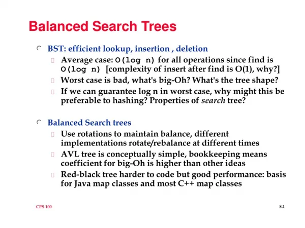
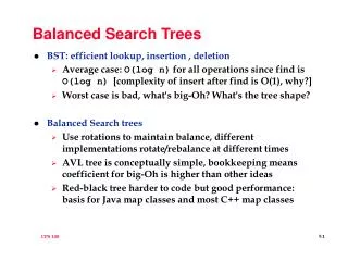
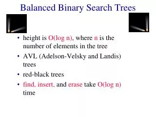
Balanced Search Trees • Definition: • Binary Search Trees with a worst-case height of O(log n) are called balanced trees • We can guarantee O(log n) performance for each search tree operation for balanced trees. • We will discuss one kinds of balanced trees: • AVL trees
AVL trees • Definition • An AVL tree is a binary search tree (BST) with an additional balance property, that is: • For any node in the tree, the height of the left subtree and the height of the right subtree differ by at most 1.
The balance property of a node • Balance information of a node t: • The balance information of a node t is given by: • balance(t) = height(t.left)-height(t.right) • A balanced tree • A binary search tree is balanced (in the AVL sense) if: • for any node t in the tree, we have • balance(t)= 0, 1 or -1
Depth property of an AVL tree • The balance condition ensures a logarithmic depth. • About the proof • In order to show that an AVL tree has a logarithmic depth, we have to show that its height h has an upper bound that is: • logarithmic in n (n is the size of the tree = the number of nodes in the tree): • h ≤ logarithmic function of n. • In other words, we need to show that: • n ≥ exponential function of h. • Therefore, we are looking for the minimum number of nodes n in an AVL tree of height h.
Theorem: the minimum number of nodes in an AVL tree • An AVL tree Thof height h has a minimum of fh+3 − 1 nodes where fh+3 is the (h + 3)th Fibonacci number. • Proof... • T his of height h: • the height of one of the subtrees of the root of Thmust be h − 1. The height of other subtree cannot be less than h − 2 (to maintain AVL balance property). Therefore, • size(Th) ≥size(Sh−1) + size(Sh−2) + 1 for h ≥ 2 (1) • where Siis the subtree of Thwith height i.
Insertion strategy in an AVL tree • The tree must be balanced before any insertion. • Insertion is performed the same way it is performed in a BST. • After an insertion, only the nodes on the path from the root to the insertion point can have their balance altered. • After a new node is inserted, we follow the path from the insertion point to the root and update the height (and balance) information of each node on that path. • If a node that violates the balance property is found, the node is re-balanced by means of a series of operations called rotations. • After a node is re-balanced and the height (or balance) information updated, no further re-balancing or updating is necessary in the remaining nodes in the path.
Possible situations after an insertion • After a new node is inserted, we follow the path from the insertion point to the root and update the height (and balance) information of each node on that path. • Say, a node X violating the balance property is found. There exist 4 possible situations: • Situation 1: the insertion is into the left sub-tree of the left child of X. • Situation 2: the insertion is into the right sub-tree of the left child of X. • Situation 3: the insertion is into the left sub-tree of the right child of X. • Situation 4: the insertion is into the right sub-tree of the right child of X.
Situation 1 An insertion into the left sub-tree of the left child of X.
Situation 2 Insertion into the right sub-tree of the left child of X.
Situation 3 (Symmetric to situation 2) Insertion into the left sub-tree of the right child of X.
Situation 4 (Symmetric to situation 1) Insertion into the right sub-tree if the right child of X.
In the following, we will consider the previous situations 2 by 2: • The first and the fourth situations are symmetric. In these situations, the insertion is performed in the left sub-tree of the left child (situation 1) of X or in the right sub-tree of the right child of X (situation 4). We call these two cases: insertion from the outside. • The second and the third situations are also symmetric. In these situations, the insertion is performed in the right sub-tree of the left child of X (situation 2) or in the left sub-tree of the right child of X (situation 3). We call these two cases: insertion from the inside.
Example: outside insertion Consider the tree on the left. After inserting 1, the tree loses its balance. We are in the situation of an outside insertion: 1 has been inserted to the left sub-tree of the left child of 8 (that lost its balance).
Example: inside insertion Consider the tree on the left. After inserting 7, the tree loses its balance. We are in the case of an inside insertion: 7 has been added to the right sub-tree of the left child of 8 (that lost its balance)
Re-balancing the tree using rotations • We have two cases: • 1 In the case of outside insertions: only a single rotation is necessary. • 2 In the case of inside insertions: a double rotation is necessary.
Single rotations: LL • Situation 1: Insertion in the left sub-tree of the left child of the node that lost balance (here X is k2). • Graphically: • LL Rotation(k2) • 1 k1 is the left child of k2. • 2 left child of k2 = right child of k1. • 3 left child of parent of k2 or right child of parent of k2 = k1 • 4 right child of k1 = k2. • 5 update height information for k2 and k1. • 6 return k1.
Pseudocode: LL rotation • Input: Binary Node k2 • Procedure withLeftChild( k2) • Set k1 k2.Left • If (k2.parent != null) • if (k2 is Left child) • k2.Parent.Leftk1 • else • k2.Parent.Right k1 • k1.parent = k2.parent • k2.parent = k1 • k2.Leftk1.Right • k1.Rightk2 • // Also, update balance information! • return k1
Single rotations: RR • Insertion in right sub-tree of right child of the node that lost • balance (Situation 4): • Graphically: • RR Rotation(k2) • 1 k1 is the right child of k2. • 2 right child of k2 = left child of k1. • 3 left child of parent of k2 or right child of parent of k2 = k1 • 4 left child of k1 = k2. • 5 update height information for k2 and k1. • 6 return k1.
Pseudocode: RR rotation • Input: Binary Node k2 • Procedure withRightChild( k2) • Set k1 k2.Right • If (k2.parent != null) • if (k2 is Left child) • k2.Parent.Leftk1 • else • k2.Parent.Right k1 • k1.parent = k2.parent • k2.parent = k1 • k2.Rightk1.Left • k1.Leftk2 • // Update balance information too! • return k1
Can we use the single rotation after an inside insertion? No we cannot!!
Double rotations: LR • Insertion in the right sub-tree of the left child of the node that • lost balance (Situation 3). • Graphically: • LR Rotation(k3) • 1 k1 is the left child of k3 • 2 k2 is the right child of k1 • 3 left child of k3 = right child of k2 • 4 right child of k1 = left child of k2 • 5 left child of parent of k3 or right child of parent of k3 = k2 • 6 left child of k2 = k1 • 7 right child of k2 = k3 • 8 update height information for k1, k3, and k2 • 9 return k2
Example of an LR rotation K3 K1 K2
Double rotation: RL • Insertion in the left sub-tree of the right child of the node that • lost balance (Situation 2): • RL Rotation(k3) • 1 k1 is the right child of k3 • 2 k2 is the left child of k1 • 3 right child of k3 = left child of k2 • 4 left child of k1 = right child of k2 • 5 left child of parent of k3 or right child of parent of k3 = k2 • 6 left child of k2 = k3 • 7 right child of k2 = k1 • 8 update height information for k1, k3, k2 • 9 return k2
In fact a double rotation is a succession of to simple rotations. • This lead to the algorithm for double rotation: • Pseudocode: LR rotation • Input: Binary Node k3 • Procedure doubleWithLeftChild( k3) • Set k3.LeftwithRightChild(k3.Left) • return withLeftChild(k3) • Pseudocode: RL rotation • Input: Binary Node k3 • Procedure doubleWithRightChild( k3) • Set k3.RightwithLeftChild(k3.Right) • return withRightChild(k3)
Deletion strategy in an AVL tree • Deletion is performed the same way it is performed in a BST. • Deleting a node from an AVL tree may cause the tree to loose its balance: one of the nodes of the tree becomes unbalanced. • After a deletion, only the nodes on the path from the root to the physically deleted node can have their balance altered. • After a new node is deleted, we follow the path from the insertion point to the root and update the height (or balance) information of each node on that path. • If a node that violates the balance property is found, the node is re-balanced by means of a series of rotations. • After a node is re-balanced and the height (or balance) information updated, no further re-balancing or updating is necessary in the remaining nodes in the path.
Possible situations after a deletion • After a node is deleted, we follow the path from the physically deleted node to the root and update the height (or balance) information of each node on that path. • Say, a node X violating the balance property is found. • There exist 6 possible situations. We will refer to these situations by: • Situation 1: deletion in the right sub-tree of X. The left child of X has a 0 balance. We refer to this situation by R0. • Situation 2: deletion in the right sub-tree of X. The left child of X has balance 1. We refer to this situation by R1. • Situation 3: deletion in the right sub-tree of X. The left child of X has balance -1. We refer to this situation by R-1. • Situation 4 (symmetric to situation 1): deletion in the left sub-tree of X. The right child of X has a 0 balance. We refer to this situation by L0. • Situation 5 (symmetric to situation 3): deletion in the left sub-tree of X. The right child of X has a 1 balance. We refer to this situation by L1. • Situation 6 (symmetric to situation 2): deletion in the left sub-tree of X. The right child of X has a -1 balance. We refer to this situation by L-1.
Situation 1: R0 Deletion in the right sub-tree of X causes X to be unbalanced. The left child of X, has balance 0. In a R0 situation, an LL rotation restores X’s balance.
Situation 1: R1 Deletion in the right sub-tree of X causes X to be unbalanced. The left child of X, has balance 1. In a R1 situation, an LL rotation restores X’s balance.
Situation 1: R-1 Deletion in the right sub-tree of X causes X to be unbalanced. The left child of X, has balance -1. In a R-1 situation, an LR rotation restores X’s balance.