Download
1 / 59
590 likes | 597 Vues
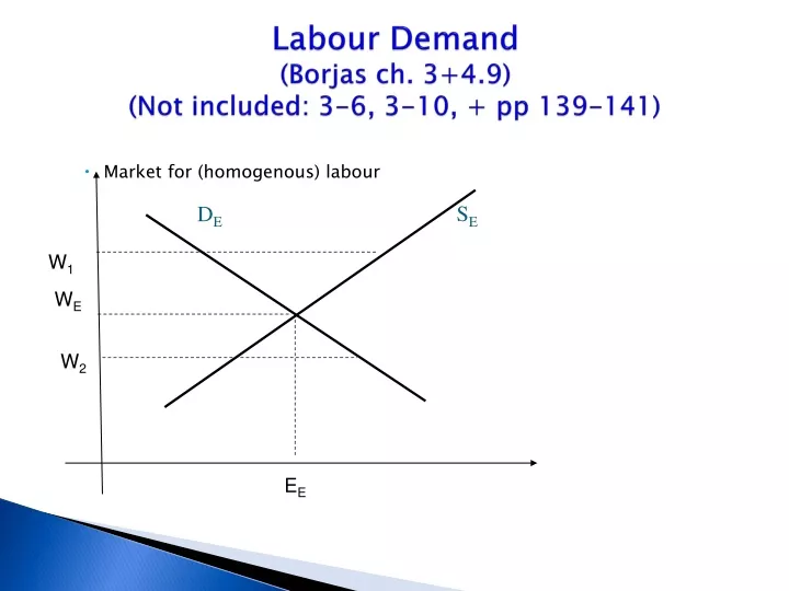
Labour Demand ( Borjas ch . 3+4.9) (Not included : 3-6, 3-10, + pp 139-141). Market for (homogenous) labour. S E. D E. W 1. W E. W 2. E E. For the seller – labour is different from other commodities. For the buyer?

E N D
Labour Demand(Borjasch. 3+4.9)(Not included: 3-6, 3-10, + pp139-141) • Market for (homogenous) labour SE DE W1 WE W2 EE
For the seller – labour is different from other commodities. • For the buyer? • Starting assumption: For the firm, labour is bought like other inputs. • Input demand is • DERIVED DEMAND not consumption demand.
Short repetition of the theory of production… • Basic assumption: • The firm hires workers in order to MAXIMISE ITS PROFITS • The firm’s demand for factors of production involves two decisions: • Produce what (how much)? • Produce how (with what technology/what inputs)?
The productionfunction • E – units of labour (hours or full time weeks or full-time worker years) • K – capital (machines, buildings, land, stocks etc.) • Production function: • Q = Q(E, K). • A more complex function would be • Q=Q(E1, E2,…, K,N,…) or Q=Q(x1, x2,…, xn)
If all other inputs are heldconstantwecanseeproduction as a function of labour. Production as a function of labour at ONE particular level of all other inputs
Marginal productivity of labour • The slope of the productionfunction shows howproductionchanges with a change in (only) labourinput. • The marginal product of labour (MPE): • The increase in productionwhen E increases by a small amount(Q(E+ΔE, K0) – Q(E, K0))/ ΔE Or mathematically • the (partial) derivative of Q with respect to E at K = K0 • At a fixedlevel of K • MPEis different at different levels of E • Marginal productivitymayincrease at small levels of E butwilleventually start to decline. • THE LAW OF DIMINISHING RETURNS
Average and marginal product If MPE > APE , APE If MPE < APE , APE MP-curve AP-curve The decreasing part of the MP-curve cuts the AP-curve in the AP-curve’s maximum
Remember: With a different level of K, we get a different Q and a different MPE for each E To each value of K corresponds another functionQ(E) and another functionMPE Analogously If labour input is constant, you can see production as a function of capital and define the marginal productivity of capital.
The employmentdecision in the shortrun = with a fixedlevel of K • VMPE = p • MPE (if the firm is a price taker in the product market) • A profit maximising firm employs until: • VMPE = MCE • Under perfect competition the firm is a ”price taker in the labour market”. • It takes w as given and MCE = w
The firm’s demand for labour Marginal revenue product of labour The marginal cost of labour (Physical) marginal product of labour The price of the product Derived demand
VMP W W2 W1 E2 E1 E Why is only the decreasing part of the VMP.curve relevant? If the ”going wage” is W2 the firm hires E2 workers – APE > MPE
Re-capitulating • Perfectcompetition: • The marginal cost of increasing E by oneunit is w • The marginal revenue of increasing E by oneunit is p •MPE • The firmincreasesemployment up to where w = p •MPE (1) • Howmany are hireddepends on • the marginal productivity of labour • the wage • the price of the product.
Ifcompetitionmight not be perfect: • In labour market: • MCE ≠ w • In product market: • MRQ ≠ p • The firm employs and produces until: • MCE = MRQ *MPE (2) • (1) is a special case of (2)
Aggregatelabourdemand in the industry(still shortrun) • Ifwagesincrease, eachemployerhiresless labour power. • Ifeachemployerhires less workers, eachemployerproducesless. • Ifallemployersproduce less, the aggregatesupplycurve for the productshifts to the left. • Equlibriumpriceincreases and the aggregatedecrease in demand for labour is less than the sum of the decreaseseachfirmwouldhavemadeif it hadbeenalonepaying the higherwage.
In the longerrun: • Both E and K can vary. • The firm has a choice between technologies. • The same output can be produced with different proportions of E and K • An ISOQUANT shows the different combinations of K and E that produce the same output
Ex: • Let be a production function. Q(64, 225) = 240 Q(144, 100) = 240 Q(72, 200) = 240 Q(200, 72) = 240 Q(100, 144) = 240 Q(225, 64) = 240 It is possible to substitute labour and capital for each other at a given level of production
Another case:Inputs are perfectcomplements Leontief production function
Standard shapeof isoquants Isoquants are negatively sloped and convex to the origin. Inputs can be substituted but MP is decreasing Q increases
MRTS • The slope of an isoquant shows how much capital is needed to replace each unit of labour without decrease in production This is the Marginal Rate of Technical Substitution, MRTS
Isocosts • An isocost shows the combinations of inputs that cost the firm the same amount. • If the cost of production is C = wE+rKthe isocosts are linear with slope –w/r K E
To maximise profits firms must: • minimise the cost of producing the chosen output • maximise production at the chosen level of cost. • This happens only at a point of tangency between an isoquant and an isocost. • These points are on the EXPANSION PATH of the firm. • Which point on the expansion path the firm chooses depends on the price of the product.
The firm will choose input combinations on the expansion path. • Each point on the expansion path represents one level of production. • The cost of inputs at that point is the minimum cost of producing that output. • The cost function of the curve C(Q) shows this minimum for each Q. • MC is the slope of this cost function – the change in cost as the firm moves outwards along the expansion path. • The firm will choose the level of production, Q*, where MC = MR and the input combination where the isoquant for Q* is tangent to an isocost
Whathappens to factoruseif w increases? (Assumeperfectcompetition & r and p constant.) • The isocostsbecomesteeper. • Morecapital intensive technology becomesmoreprofitable. • At everypoint on everyisoquant, cost and marginal costincreases. • The MC-curvemovesupwards-leftwards. • The firmwilldecreaseproduction. It willchoose the tangencypoint of anotherisoquant with anotherisocost.
A wageincrease has twoeffects on employment: • 1. Changed relative priceswill make the firmchange the capital/labourratio • 2. Changed MC will make the firmdecrease output. Decreased output will make the firmuse less inputs. Therewill be SUBSTITUTION EFFECTS and SCALE EFFECTS
Employment when w increases P is choice with lower wage R is choice with new higher wage E*-E1 is scale effect E2-E* is substitution effect P R S Q1 Q2 E2 E* E1
Use of capital when w increases P is choice with lower wage R is choice with new higher wage K*-K1 is scale effect K2-K* is substitution effect K2 P K1 R S Q1 K* Q2
w, r constant • If both capital and labour are ”normal” inputs the scale effects of both are negative. • The substitution effect increases K and decreases E. • The total effect on E must be negative, the total effect on K depends on the size of the effects.
Elasticity of labour demand: The long run labour demand elasticity > short run labour demand elasticity Estimates of labour demand elasticity vary depending on the time and place, the level of aggregation, the method used (assumptions about production the function) Hamermesh’s survey: Many studies find ε -0.3 Swedish studies (Ekberg, Walfridsson) -0.3 & -0.2 Scale effects included: -0.65 Lower elasticity for highly educated workers Lower for white collar than for blue collar Higher for young than for older workers
Elasticity of substitution: • The elasticity of substitution between two factors of production is The size depends on the shape of the isoquants. • If they are perfect substitutes a change in relative price leads to no change at all or a total switch • If they are perfect complements, the elasticity is zero. qi,and pi are quantitites and prices of the two inputs
Empirical estimates of capital/labour substitution elasticities vary: • For whole or large parts of economies 0-1, most often 0.4-0.8 • Swedish estimates: wide range at different times and different industries and different for different groups of workers.
With many inputs:Q=Q(E1, E2,…, K,N,…) • Factor i will be employed at the level where VMPi=MPi*p • If the price of one factor goes up, what happens to demand for the others? • The cross-elasticity of demand between factor i and k =
If δik< 0 factors i and k are complements in production • An increase in the price of k shifts the demand curve for i leftwards • If δik> 0factors i and k are substitutes in production • An increase in the price of k shifts the demand curve for i rightwards
Empirical studies: • Many studies find that skilled labour (or white collar) and capital are complements while unskilled (or blue collar) labour and capital are substitutes. • Worker groups with different skills and characteristics can be substitutes or complements.
Marshall’s rules: • Demand for labour/one type of labour is less elastic: • If it is very essential to production and difficult to replace either by capital or other labour. • If demand for the final product is inelastic. • Their wages make up a small part of total costs of production. • If the supply of complements to it is inelastic and that of substitutes elastic. The less elastic demand is, the greater the scope for unions to increase wages with small loss in employment.
Why “If the supply of complements to it is inelastic and that of substituteselastic.“ • Assume: Two groups of workers, A & B, are complements • wages of group A demand for both groups • Demand for labour of type B their wage wB . If supply is inelastic, wB much and the firm reduces output less. • Assume: Labour of type A and capital are substitutes. • wA firm wants to substitute capital for labour • If supply of capital is elastic, increase in demand price of capital , reducing the incentives for the firm of substituting from labour to capital
Two groups of workers, A & B, are complements D1 Inelastic supply Elastic supply D2
Labour market structure and labour demand • Perfect competition W W2 VMP W1 E2 E1 E
Monopsony MCEW • Can occur due to: • A very restricted local labour market (”company town”, ”bruksort”) • Very high degree of specialisation (perhaps unique to the firm) • Segregation/discrimination • Monopoly (public or private)
A discriminating monopsonist pays each worker his/her reservation wage. Employment is = EPerfect comp. but all workers except the last get less than wPC • A non-discriminating monopsonist pays all workers the same wage. Therefore the cost of hiring an additional worker > the wage of that worker (if labour supply is upward sloping). Both employment and wage will be less than under perfect competion.
Labour demand with (non-discriminating) monopsonist: W W MCE LS WPC WM VMP EM EPC E
Minimum wages • Can be set by legislation or in collective agreements. • Effects: • On distribution of income (tend to equalise) • On employment (usually negative but the evidence is mixed and disputed). • Encourages structural change
SL SL Labour supply with and without minimum wage
MLC Wmin S S VMP Effects of minimum wage under perfect competition and monopsony Monopsony Perfect competition: VMP Employment Wage Unemployment Employment Wage Unemployment
A firm dominates employment in a small town. The price of its product is 10 SEK. The firm’s production function is : Q = 20E – 0.005 E2 • Q = production • E = Employment. • a) What is the firm’s labour demand function DE ? • What is its labour demand if w= 150 SEK? • b) Assume that the firm is a monopsonist in this labour market and that labour supply is given by. • w=50+0.2E • What is MCE • Calculate the firm’s DE and the wage, w. • c) The state sets a minimum wage w=150, How many workers will the firm employ? • a) VMPE=p*MPE=10*(20-0,01E)=200-0,1E • Profit maximisation requires that VMPE=MCE=w • DE is given by: w=200-0,1E E=2000-10w • w=150 => E=500 • b) The labour cost of the firm : • E*w = E*(50+0.2E) = 50E+0.2E2 • MC E : 50+0.4E • MC E =MRP E50+0.4E= 200-0.1E • E = 300 • To employ 300 workers the firm has to pay • w=50+0.2L=50+60=110 • c) With a minimum wage S E =0 for w<150 • MC E =150 • ´Profit maximisation requires that VMP E =150 =>E=500
Adjustment costs – labour as a quasifixed factor of production • Transaction costs • Search and hiring costs • Training costs for new employees • Severance pay • Negotiations, law suits • Loyalty, work climate • Reputation as an employer • Uncertainty about how lasting and how big an up/downturn in product demand/business cycle will be.