Download
1 / 30
300 likes | 416 Vues
Strategies to solve the rendering or potential equations. L ászló Szirmay-Kalos. Coupling in the rendering equation. L (x, w )= L e ( x, w )+ L ( h ( x,- w) , w ) f r ( ’ ,x, ) cos ’ d w ’. L ( h ( x,- w) , w ). h ( x,- w). L (x, w ). ’. ’. w. x. f r ( ’ ,x, ).

E N D
Strategies to solve the rendering or potential equations László Szirmay-Kalos
Coupling in the rendering equation L(x,w)=Le(x,w)+L(h(x,-w),w)fr (’,x,) cos ’dw’ L(h(x,-w),w) h(x,-w) L(x,w) ’ ’ w x fr (’,x,)
Compromises in the solution • Ignore all types of coupling: • local illumination models • Follow just very specific types of coupling that have finite number: • recursive ray-tracing • Resolve the coupling: • global illumination models
Example: x = 0.1 x + 1.8Solution by ignoring the coupling • Ignoring the coupling: • right side’s x: x = 0.1 x + 1.8 1.8 • Approximate solution: • x = 0.1·1.8 + 1.9 = 1.98
Local illumination models • The radiance of in the right side: • is replaced by an approximation of the emission function: abstract lightsources • Single reflection of the light from the abstract lightsources are computed L(x,w)=Le(x,w)+Llightsource fr (’,x,) cos ’dw’ Le(x,w)
Lightsource models • Ambient lightsource: La constant • ambient refl. model: Lref = La ka • Sky-light model: Lref = La a(x, view dir) • Directional lightsource • radiates into a single direction, the intensity is independent of the position • Positional lightsource • radiates from a single position, the intensity decreases with the square distance
Local illumination algorithms pixel • Visibility computation from the eye • Lightsource visibility from the visible point • Calculation of the reflection of the light from the lightsources
Result of local illumination models Without lightsource visibility computation With lightsource visibility computation
Recursive ray-tracing • The radiance of in the right side is replaced by an approximation of the emission function and by the radiance from ideal refraction and refraction directions • Single incoherent reflection and multiple coherent reflections of the light from the abstract lightsources are computed L(x,w)=Le(x,w)+ + Llightsource fr (’,x,) cos ’dw’ + krLin (x, wr) + ktLin(x, wt)
refracted ray reflected ray shadow rays Llightsource Recursive ray-tracing
Comparison of the solution alternatives of L = Le +tL Local illumination with shadows 0.1 sec … sec Recursive ray tracing secs… mins Global illumination mins … hours
Global illumination solution • Inversion • Expansion • Iteration (1- )L = Le L = (1- ) -1Le L = Le+L = Le+Le+2L= Le+Le+2 Le +3L = nLe Ln = Le+ Ln-1
Example: x = 0.1 x + 1.8Solution by inversion • Grouping the unknown terms: • 0.9 x = 1.8 • Inversion: • x = 0.9 -1 1.8 = 2 • Luck: multiplication by a scalar is invertible
Inversion (1- )L = Le L = (1- ) -1Le • is infinite dimensional • it requires finite approx. of and the radiance L : • finite element techniques
Example: x = 0.1 x + 1.8Solution by expansion • xi=1.8+0.1 1.8 +0.121.8 + …+ 0.1i+1x • i: 1 2 3 4 • xi sequence: 1.8 1.98 1.998 1.9998
Expansion L=Le+L=Le+Le+2L=nLe ifnL 0 • should be a contraction • Rendering equation: • radiance: • measured power: • Potential equation: • potential: • measured power: L = nLe F= ML = M nLe W = ’ n We F= M’W = M’ nWe
Error of truncating the Neumann series ML = M nLe DM nLe error= |n=D+1M nLe |=|M D+1( n=0 nLe )| qD+1F || L|| q||L||, q is the contraction
Terms of the expansion of the rendering equation: 1-bounce M(Le) = P R(p,w1) Le(y,-w1) dw1dp Le y L(x,w) ’1 w1 w p x R(p,w1) = 1/Spfr (w1,x,) cos’1
Terms of the expansion of the rendering equation: 2-bounce M(2Le)=P R(p,w1,w2)Le(z,-w2) dw1dw2dp Gathering walks y w2 L(x,w) ’1 z ’2 w1 w p x Le R(p,w1,w2) = 1/Spfr (w1,x,)cos’1 fr (w2,y,1)cos’2
Terms of the expansion of the potential equation: 1-bounce M’(’We)= S Le(x,w)cos{ We(y,w1) fr(w,y,1)cos1dw1 }dwdx = S Le(x,w)cosfr(w,y,eye)g(y)dwdx=S Le(x,w)R(x,w)dwdx x w Le (x,w) p 1 weye y R(x,w) = cos fr (w,y,eye) g(y)
Terms of the expansion of the potential equation: 2-bounce F=M’(’2We)=S R(x,w,w1) Le(x,w) dw1dwdx Shooting walks y w1 p x 2 1 w weye z Le (x,w) R(x,w,w1) = cos fr (w,y,1)cos1 fr (w1,z,eye) c(p)
Expansion is a series of high dimensional integrals R(w1,...,wn,x) = w1 w2 …wn wi= fr cos ’ pixel w 1 e w L 2 F=n...R(w1,...,wn,x)Le(w1,...,wn,x)dw1,...,dwndx 1/M iM nDR(w1(i),...,wn(i),x(i) )Le(w1(i),...,wn(i),x(i)) • It requires just discrete samples from Le and R • No finite elements are needed
Example: x = 0.1 x + 1.8Solution by iteration • Iteration scheme: • xn = 0.1 xn-1 + 1.8, • n: 1 2 3 4 • xnsequence:0 1.8 1.98 1.998 1.9998
Iteration Ln = Le+ Ln-1 • Requirements of convergence • Convergent: Ln = Le+ Ln-1 Ln -1 = Le+ Ln-2 |Ln-Ln-1| = |(Ln-1-Ln-2)| = |n-1(L1-L0)| lim |n-1(L1-L0)| = 0
If is a contraction • || L || q||L||, • q < 1contraction ratio = albedo • ||n-1(L1-L0) || q n-1||L1-L0|| • converges with the speed of the geometric series e.g.: • ||L||1=, q is the average albedo
Error analysis of the iteration • Assume that is only approximated by * • L1 = Le+* L= L+L • L2 = Le+* L1 = L+L+* L • … • Ln = Le+* Ln-1 = L+L+*L+*2 L+... • ||L-L||||L||+||*L||+…=||L||(1+q+q2+…) ||L-L|| || L- * L || / (1-q)
Analitically solvable cases • Normal approach: scene radiance solution • Inverse approach: radiance scene • Good for testing global illumination algorithms • constant radiance • constant reflected radiance
Constant radiance L (x,w) = L* L*= Le (x,w)+tL* = Le (x,w)+L*t1 = Le (x,w)+L* a(x,w) • a(x,w) = 1 - Le (x,w)/ L* • arbitrary geometry in a closed environment
Constant reflected radiance L (x,w) = Le (x,w)+Lr* Le +Lr* = Le +t(Le +Lr* ) = Le +t(Le +Lr* )= Le +tLe +Lr*t1 = Le +tLe +Lr*a(x,w) • a(x,w) = 1 - tLe(x,w)/ Lr* • special case: constant albedo?
R y x’ y x |x-y| Spherical geometry with diffuse emission: constant reflected radiance tLe= Le(h(x,-w’)) fr cosx’ dw’ = S fr cosx’ cosyLe(y)/|x-y|2 dy cosx’=cosy=|x-y|/2R tLe=fr S Le(y) dy 4R2 =albedo average(Le)