Download
1 / 17
170 likes | 330 Vues
Lecture 4: Cross sections. Review distributions (SI, SP) Finish source/beam distributions New MCNP command: En Interpolation: xxi Vised skills: Plotting source points Plotting cross section MCNP cross section estimation Neutron: Total, absorption, scattered energy

E N D
Lecture 4: Cross sections • Review distributions (SI, SP) • Finish source/beam distributions • New MCNP command: • En • Interpolation: xxi • Vised skills: • Plotting source points • Plotting cross section • MCNP cross section estimation • Neutron: Total, absorption, scattered energy • As time permits=>Source distributions
X axis of a distribution: SI Syntax: Description: The SIn and SPn cards work together to define a pdf to select a variable from. option= blank or Hhistogram =Ldiscrete =A(x,y) pairs interpolated =Sother distribution #’s
Y axis of a distribution: SP • Syntax: • Description: Specification of y axis of pdf for distribution n. • option=blankcompletes SI • =-ppredefined function • The P values are the y-axis values OR the parameters for the desired function p—and the SI numbers are the lower and upper limits • The predefined distribution we will use most often is 21: • SIxxrlowrhigh • SP -21 exponent
Examples SI2 H 0 5 20 SP2 0 1 2 … SI3 L 1 2 SP3 1 2 … SI4 A 0 5 20 SP4 0 1 2 … SI5 1 5 SP5 –21 2
Source description variables • Commands: • POS=Position of a point of interest • RAD=How to choose radial point • AXS=Direction vector of an axis • EXT=How to choose point along a vector • X,Y,Z=How to choose (x,y,z) dimensions • VEC=Vector of interest • DIR=Direction cosine vs. VEC vector • Combinations: • X,Y,Z: Cartesian (cuboid) shape • POS, RAD: Spherical shape • POS, RAD, AXS, EXT: Cylindrical shape • VEC,DIR: Direction of particle
Volumetric/beam sources • Cuboid sources: • X,Y,Z=How to choose (x,y,z) dimensions • Spherical sources • POS=Position of the sphere center • RAD=How to choose radial point (usually a distribution using -21 2) • Cylindrical sources • POS=Position of base of the cylinder • AXS=Direction vector of an axis • EXT=How to choose point along a vector • RAD=How to choose radial point • Beam source • POS=Position of the source center • VEC=Vector of direction of the beam • DIR=Direction cosine vs. VEC vector (distirbution or just 1.0)
Other source shapes • If you have a shape OTHER than one of the three allowed (sphere, cuboid, cylinder), you can • Create a cell in your problem that has the shape you want • Create a volumetric source (sphere, cuboid, or cylinder) that COMPLETELY ENCLOSES the cell you created in the previous step • Add CEL=xxx to the SDEF card, with the cell number of the cell you created
Energy bins: En • Syntax: • Description: Create energy UPPER ranges from LOW to HIGH • MCNP5 Manual Page: 3-96
MCNP skill: Interpolation 1 2 3 4 5 6 … 99 100 can be replaced (saving typing) with interpolation: 1 98i 100 The number before the “i” is how many numbers to add, NOT how many divisions there are!
VisEd skill: Plotting source points • Create the input file • Open VisEd to view the geometry • Zoom in or out/translate axis as desired to give you the view you want • Click anywhere inside the view you want to source particles to appear in • Under the main toolbar “Particle display” choose “Plot Particle Tracks” • A window of choices will pop up • Move the new popup window out of the way, if you want • Choose: • Number of particles to plot: Play with this to get the density of particles you want • Distance from plot plane: This is how far off the plane the particle can be (into or out of the screen) and still be plotted • Display: Source (For this exercise only. You can make other choices to see collisions, etc.) • Click on “Plot_Source” on popup toolbar • Example: EX3A
VisEd skill: Plotting cross sections • Create input file • Open VisEd • Click toolbar “Cross Section Plots” • A popup window will appear • Click “Read_Cross_Sections” from popup toolbar • Beside “Nuclide” (you could also plot material cross sections using “Material”): • Enter a number in the box and press “Plot” • It will NOT plot anything, but the error message will tell you which “zaids” it knows about • Pick the one you want and type it into the box (including any suffix, e.g., “.70c”) • From the pull-down menu that is under the “Nuclide” box (it probably says “1 Total (N)” in it) and pick the reaction you want it to plot • Absorption is way down the list at 101 • Photon cross sections start at 501 • The inelastic neutron cross sections start at 51 • Press “Plot” again. It will show up in the active window • Example: EX4A
HW 3.5 • Use an MCNP calculation of a beam impinging on the small water sample to estimate the total cross section of water for 0.1 MeV, 1 MeV, and 10 MeV photons. Compare your answers to the values in Appendix C of the text.
HW 4.1 • What is the maximum possible fracitonal energy loss from Compton scattering for initial photon energies of 0.1, 1., 10, and 100 MeV? • What is the threshold neutron energy to excite the second level of Pb-207? If a 1 MeV neutron excites this level, what is the energy range for possible particle energies after the collision? • What is the energy range for possible particle energies after an elastic collision of a 1 MeV neutron with Pb-207?
HW 4.2 • The energy ranges for each of the three photon mechanisms—photoelectric effect, Compton scattering, and pair production—given in the lesson were approximate. Use Table C.5 to find the true dominance range (i.e., for each mechanism, the energy range over which it is the largest component of mu) for all five materials in the table: air, water, concrete, iron, and lead.
HW 4.3 • For a 0.1 MeV neutron impinging on a small B-10 source, use an MCNP calculation like that used in class (beam impinging on the end of a very thin cylinder enclosed in an F1/E1-tallying sphere) to estimate: • Total microscopic cross section • Elastic scattering cross section • Absorption cross section • Check your results using the VisEd cross-section viewer
HW 4.4 • For a 1 MeV neutron impinging on a small B-10 source, use an MCNP calculation like that used in class (beam impinging on the end of a very thin cylinder enclosed in an F1/E1-tallying sphere) to estimate: • Total microscopic cross section • Elastic scattering cross section • Absorption cross section • Inelastic cross section and Q value • Check your results using the VisEd cross-section viewer and Table 3.1 in the text
HW 4.5 • For a 10 MeV photon impinging on a small Lead source, use an MCNP calculation like that used in class (beam impinging on the end of a very thin cylinder enclosed in an F1/E1-tallying sphere) to estimate: • mt • mpp • Check your results using the VisEd cross-section viewer OR comparing to Table C.5 in the text