Download
1 / 20
260 likes | 516 Vues
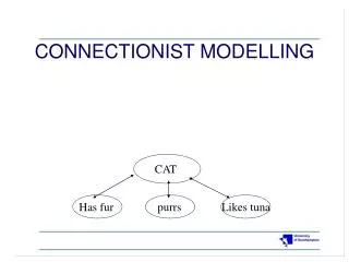
Connectionist models. Connectionist Models. Motivated by Brain rather than Mind A large number of very simple processing elements A large number of weighted connections between elements (network) Parallel, distributed control Emphasis on learning internal representations automatically.

E N D
Connectionist Models • Motivated by Brain rather than Mind • A large number of very simple processing elements • A large number of weighted connections between elements (network) • Parallel, distributed control • Emphasis on learning internal representations automatically
The Perceptron Output unit w0 w1 w3 w2 Bias unit Input units 1 x1 x2 x3
Training the Perceptron I • The original idea here was to train the perceptron by changing the weights in accordance with experience – designed to mimic the real life neuron. • If the classification was correct then the weights are unchanged,, however if the classification was wrong then the weights are altered
Training the Perceptron II • The weights are altered according to a simple rule: New wi = Old wi +(t-y)xi Here the true outcome is t, the predicted outcome is y, and is the learning rate.
The Method Works! • For linearly separable data the method works and will give a line that separates the data into two sets. • Even better the method can be proved to work! • However for data which is not linearly separable the method does not converge.
Neural Nets • The Neural Net is a development from the Perceptron in that several Perceptrons are linked together in a net. • Also the threshold function (used in the output unit) is often changed to a continuous function like the logistic function. • This leads to a variety of possible architectures.
Multilayered Networks • Input layer • Hidden layer 1 • Hidden layer 2 ... • Hidden layer N • Output layer • Each layer is fully connected to its preceding and succeeding layers only • Every connection has its own weight
•Each node at next layer will compute the sigmoid function and propagate values to the next layer •Propagate these values forward until output is achieved
Neural Net +1 +1 Bias Units wij Outputs Inputs Hidden Layer(s)
Neural Net Theory • A Neural Net with no hidden layers can classify linearly separable problems • A neural net with one hidden layer can describe any continuous function • A neural net with two hidden layers can describe any function
Back Propagtion • After early interest Neural Nets (NN’s) went into decline as people realized that while you could train perceptrons successfully, this only worked for linearly separable data and no-one had a method to train nets with a hidden layer. • The method was suggested by Werbos(1974) but the modern form was given by Rumelhart and McClelland in 1986. The technique is based on gradient search techniques.
Backpropagation • To train a multilayered network: • randomly initialize all weights [-1..+1] • choose a training example and use feedforward • if correct, backpropagate reward by increasing weights that led to correct output • if incorrect, backpropagate punishment by decreasing weights that led to incorrect output
Backpropagation continued • Continue this for each example in training set • This is 1 epoch • After 1 complete epoch, repeat process • Repeat until network has reached a stable state (i.e. changes to weights are always less than some minimum amount that is trivial) • Training may take 1000’s or more epochs! (even millions)
Uses of NNs • NN are knowledge poor and have internal representations that are meaningless to us • However, NN can learn classifications and recognitions • Some useful applications include • Pattern recognizers, associative memories, pattern transformers, dynamic transformers
Particular Domains • Speech recognition (vowel distinction) • Visual Recognition • Combinatorial problems • Motor-type problems (including vehicular control) • Classification-type problems with reasonable sized inputs • Game playing (backgammon)
Advantages of NN • Able to handle fuzziness • Able to handle degraded inputs and ambiguity • Able to learn their own internal representations & learn new things • Use distributed representations • Capable of supervised & unsupervised learning • “Easy” to build
Using R to implement Neural Nets • R only fits neural nets with one hidden layer • There are two ways of fitting neural nets to data in R • Via the “model” format NNB.nn2 <- nnet(Type ~ x+y, data = NNeighbour, subset = samp, size = 2, rang = 0.1, decay = 5e-4, maxit = 200)
Using R to implement Neural Nets 2 2. And via the “data” method: NNB.nn1 <- nnet(NNB[samp,], Ntype[samp], size = 2, rang = 0.1, decay = 5e-4, maxit = 200) Note for this method the data needs to be numeric – even the classification data
Using R to implement Neural Nets 3 • R uses a random allocation of weights before training the network so each time you perform the calculation you will get different answers • It is easy in R to select a sample of the data and to train the data on that sample: Just use the “sample(1:50,25)” function which will select 25 cases at Random from the first 50 cases