Download
1 / 18
180 likes | 265 Vues
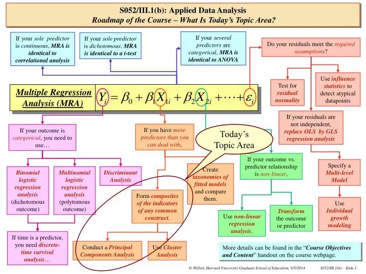
If your several predictors are categorical , MRA is identical to ANOVA. If your sole predictor is continuous , MRA is identical to correlational analysis. If your sole predictor is dichotomous , MRA is identical to a t-test. Do your residuals meet the required assumptions ?.

E N D
If your several predictors are categorical, MRA is identical to ANOVA If your sole predictor is continuous, MRA is identical to correlational analysis If your solepredictor is dichotomous, MRA is identical to a t-test Do your residuals meet the required assumptions? Use influence statistics to detect atypical datapoints Test for residual normality Multiple Regression Analysis (MRA) If your residuals are not independent, replace OLS byGLS regression analysis If you have more predictors than you can deal with, If your outcome is categorical, you need to use… Today’s Topic Area If your outcome vs. predictor relationship isnon-linear, Specify a Multi-level Model Create taxonomies of fitted models and compare them. Binomiallogistic regression analysis (dichotomous outcome) Multinomial logistic regression analysis (polytomous outcome) Discriminant Analysis Form composites of the indicators of any common construct. Use Individual growth modeling Transform the outcome or predictor Use non-linear regression analysis. If time is a predictor, you need discrete-time survival analysis… Conduct a Principal Components Analysis Use Cluster Analysis S052/III.1(b):Applied Data AnalysisRoadmap of the Course – What Is Today’s Topic Area? More details can be found in the “Course Objectives and Content” handout on the course webpage.
Today, in Sections III.1(b) & (c) on Using Principal Components Analysis, I will: • Introduce the idea of forming a general weighted linear compositefrom multiple indicators. • Show how Principal Components Analysis can create an optimal weighted linear composite. • Identify the 1st principal component as the required optimal composite. • Interpret the 1st principal component by inspecting weights in the 1st eigenvector. • Determine the variance of the 1st principal component by examining the1st eigenvalue. • Connect the dimensionality of a set of indicators to the eigenvalues produced by PCA. • Determine the dimensionality of a set of indicators using Rule of One & Scree Plot. • Appendix 1: Assessing the magnitudes of the elements of the eigenvector S052/III.1(b):Using PCA To Form An “Ideal” Composite From Multiple IndicatorsPrinted Syllabus – What Is Today’s Topic? Please check inter-connections among the Roadmap, the Daily Topic Area, the Printed Syllabus, and the content of today’s class when you pre-read the day’s materials.
S052/III.1(b):Using PCA To Form An “Ideal” Composite From Multiple IndicatorsRecalling the TSUCCESS Dataset • A dataset in which the investigators measured multiple indicators of what they thought was a single underlying construct that represented Teacher Job Satisfaction: • The data described in TSUCCESS_info.pdf.
A standardized composite is formed by first standardizing each indicator to zero mean & standard deviation 1: Then, the standardized indicator scores are added together to form composite Ci, as follows: Or, if you prefer to use “normed” weights, Ci would be†: † Weights are said to be “normed” when the sum of their squares is equal to one. S052/III.1(b):Using PCA To Form An “Ideal” Composite From Multiple IndicatorsExtending The Basic “Equally-Weighted” Standardized Composite I have argued that, when forming composites, a standardized composite is preferred, to compensate for the heterogeneous metricsandvariances of the multiple indicators being composited, as follows … Cronbach Coefficient Alpha Variables Alpha ƒƒƒƒƒƒƒƒƒƒƒƒƒƒƒƒƒƒƒƒƒƒƒƒƒƒƒƒ Raw 0.696594 Standardized 0.735530
By choosing weights that differ from unity and differ from each other, we can create an infinite number of potential composites, as follows: • Where we typically use “normed” weights, such that: • Among all such weighted linear composites, are there some that are “optimal”? • How would we define such “optimal” composites?: • Does it make sense, for instance, to seeka composite with maximum variance, given the original standardized indicators. • Perhaps I can also choose weights that take account of the differing inter-correlations among the indicators, and “pull” the composite “closer” to the more highly-correlated indicators? S052/III.1(b):Using PCA To Form An “Ideal” Composite From Multiple IndicatorsAn Extension Of The Basic Standardized Composite To Include “Weights”? More generally, a weighted linear composite can be formed by weightingandaddingstandardizedindicators together to form a composite measure of teacher job satisfaction … Cronbach Coefficient Alpha Variables Alpha ƒƒƒƒƒƒƒƒƒƒƒƒƒƒƒƒƒƒƒƒƒƒƒƒƒƒƒƒ Raw 0.696594 Standardized 0.735530
PROC PRINCOMP is the PC-SAS procedure for conducting Principal Components Analysis (PCA): • By choosing sets of weights, PCA seeks out optimal weighted linear composites of the original standardized indicators. • These composites are called the “principal components.” • The first principal component is that weighted linear composite that has maximum variance, given the indicator-indicator inter-correlations. The VAR statement specifies the indicators to include in the PCA • After a PCA, scores on thenew composite(s) are output, for each person, and you must: • Specify adataset into which they are output (here, I used the original dataset, TSUCCESS). • Provide a prefix to be used for labeling the new composite variable(s) (here, PC_ ). S052/III.1(b):Using PCA To Form An “Ideal” Composite From Multiple IndicatorsProgramming Principle Components Analysis In PC-SAS In Data-Analytic Handout III.1(b).1… *-----------------------------------------------------------------------------* Input the dataset, name and label the six indicators of teacher satisfaction *-----------------------------------------------------------------------------*; DATA TSUCCESS; INFILE 'C:\DATA\S052\TSUCCESS.txt'; INPUT X1-X6; LABEL X1 = 'Have high standards of teaching' X2 = 'Continually learning on job' X3 = 'Successful in educating students' X4 = 'Waste of time to do best as teacher' X5 = 'Look forward to working at school' X6 = 'Time satisfied with job'; PROC FORMAT; VALUE AFMT 1='Strongly disagree' 2='Disagree' 3='Slightly disagree' 4='Slightly agree' 5='Agree' 6='Strongly agree'; VALUE BFMT 1='Strongly agree' 2='Agree' 3='Slightly agree' 4='Slightly disagree' 5='Disagree' 6='Strongly disagree'; VALUE CFMT 1='Not successful' 2='Somewhat successful' 3='Successful' 4='Very Successful'; VALUE DFMT 1='Almost never' 2='Sometimes' 3='Almost always' 4='Always'; *-----------------------------------------------------------------------------* Carry out the principal components analysis *-----------------------------------------------------------------------------*; PROC PRINCOMP DATA=TSUCCESS OUT=TSUCCESS PREFIX=PC_; VAR X1-X6;
Notice the sample size used in the PCA: • Recall that the total sample size was 5269 teachers. • PCA has used thelist-wise deletedsample of 4955 teachers in order to avoidviolations of positive definiteness. X4 X5 X6 4.2270 4.4244 2.8365 1.6660 1.3289 0.5714 The PRINCOMP Procedure Observations 4955 Variables 6 Simple Statistics X1 X2 X3 Mean 4.3294 3.8736 3.1550 StD 1.0882 1.2427 0.6693 • As a first step, PCA estimates the sample meanandstandard deviation of the indicators and standardizes each of them automatically, as follows: • So, we begin with a total ofsix unitsof originalstandardized indicator variancethat PCA then seeks todisperse maximally into new composites. S052/III.1(b):Using PCA To Form An “Ideal” Composite From Multiple IndicatorsPCA Provides Univariate Output … The output has several important features, starting with ...
PCA assumes that all bivariate inter-relationships among the indicators are linear-- so, in a thorough PCA, you must: • Check the bivariate linearity assumption by inspecting a complete set of bivariate scatter-plots (not included here). • Fix any curvilinearity by applying suitable transformations to the indicators before proceeding (not needed here). Procedure Variables 6 X2 X3 X4 X5 X6 0.5548 0.1610 0.2127 0.2531 0.1921 1.0000 0.1663 0.2313 0.2697 0.2225 0.1663 1.0000 0.2990 0.3557 0.4326 0.2313 0.2990 1.0000 0.4478 0.3993 0.2697 0.3557 0.4478 1.0000 0.5529 0.2225 0.4326 0.3993 0.5529 1.0000 The PRINCOMP Observations 4955 Correlation Matrix X1 X1 Have high standards of teaching 1.0000 X2 Continually learning on job 0.5548 X3 Successful in educating students 0.1610 X4 Waste of time to do best as teacher 0.2127 X5 Look forward to working at school 0.2531 X6 Time satisfied with job 0.1921 PCA seeksaset ofideal compositesthat are mutually uncorrelated and with decreasingmaximum variance, given the set of original indicators: • Of course, it may not succeed in piling all six units of original standardized variance into a single “ideal” composite because the original indicators are not all perfectly inter-correlated to begin with! • So, in creating its “ideal composites,” PCA accounts for inter-correlations among the indicators, putting as much of original variance into the 1st component as it can, before moving on to the creation of the 2nd, etc. S052/III.1(b):Using PCA To Form An “Ideal” Composite From Multiple IndicatorsPCA Provides Bivariate Output …
Eigenvectors PC_1 PC_2 X1 Have high standards of teaching 0.3472 0.6182 X2 Continually learning on job 0.3617 0.5950 X3 Successful in educating students 0.3778 -.3021 X4 Waste of time to do best as teacher 0.4144 -.1807 X5 Look forward to working at school 0.4727 -.2067 X6 Time satisfied with job 0.4591 -.3117 PC_3 PC_4 PC_5 PC_6 0.0896 0.0264 0.6261 0.3108 0.0543 -.0217 -.6685 -.2548 0.7555 0.4028 0.0503 -.1746 -.5972 0.6510 -.0493 0.1129 -.2418 -.4501 0.3022 -.6176 0.0558 -.4584 -.2548 0.6433 .35 First principal component This Column Is Called The “First Eigenvector” It contains the weights that PCA has determined will provide a linear composite of the six original standardized indicators with maximum possible variance, given the inter-correlations among the indicators. .36 .38 This “ideal” composite is called the first principal component, it is: Where: .41 .47 .46 S052/III.1(b):Using PCA To Form An “Ideal” Composite From Multiple IndicatorsPCA Provides Multivariate Output … List of the original indicators
PC_1 PC_2 X1 Have high standards of teaching 0.3472 0.6182 X2 Continually learning on job 0.3617 0.5950 X3 Successful in educating students 0.3778 -.3021 X4 Waste of time to do best as teacher 0.4144 -.1807 X5 Look forward to working at school 0.4727 -.2067 X6 Time satisfied with job 0.4591 -.3117 PC_3 PC_4 PC_5 PC_6 0.0896 0.0264 0.6261 0.3108 0.0543 -.0217 -.6685 -.2548 0.7555 0.4028 0.0503 -.1746 -.5972 0.6510 -.0493 0.1129 -.2418 -.4501 0.3022 -.6176 0.0558 -.4584 -.2548 0.6433 • Each standardized indicator is approximately equally weighted in the First Principal Component: • This suggests that the first principal component is an even-handed synthesis of information originally contained equally in the six original standardized indicators. • Teachers who score highly on the first principal component: • Have high standards of teaching performance. • Feel that they are continually learning on the job. • Believe that they are successful in educating students. • Feel that it is not a waste of time to be a teacher. • Look forward to working at school. • Are always satisfied on the job. • Let’s define the first principal component as anoverall index of teacher enthusiasm? First principalcomponent .35 .36 .38 .41 .47 .46 S052/III.1(b):Using PCA To Form An “Ideal” Composite From Multiple IndicatorsWhat Is The First Principal Component Measuring?
The eigenvalue for the first principal component is its estimated variance: • In this example, where indicator-indicator correlations were low, the best that PCA has been able to do is to form an “optimal” composite that contains 2.61 units of standardized variance, out of the original 6 units. • That’s 43.43% of the total original standardized variance. • This impliesthat 3.39 units of the original standardized variance remaining may measure something else!!! • Perhaps we can form other substantively-interesting composites from these same six indicators, by choosing different sets of weights: • Maybe there are other “dimensions” of information still hidden within the data? • Let’s inspect the other “principal components” that PCA has formed in these data … This column contains the eigenvalues. S052/III.1(b):Using PCA To Form An “Ideal” Composite From Multiple IndicatorsHow Much Of The Original Standardized Variance Does The 1st Component Contain? Eigenvalues of the Correlation Matrix Eigenvalue Difference Proportion Cumulative 1 2.60599489 1.39439026 0.4343 0.4343 2 1.21160463 0.49880170 0.2019 0.6363 3 0.71280293 0.11761825 0.1188 0.7551 4 0.59518468 0.14741881 0.0992 0.8543 5 0.44776587 0.02111886 0.0746 0.9289 6 0.42664701 0.0711 1.0000
What’s going on here is that PCA has piled as much of the 6 units of original standardized variance as it can into the first principal component(43%) and created a composite with maximum possible variance (2.61 units), given these indicators • Then, it has taken the remaining variance (3.31 units or 57%) and used as much of it as possible to form a second principal component, that: • Is uncorrelated with the first component, • Has the next largest possible variance (1.21 units or an additional 20.19%). Then, it’s done the same again with a third principal component…. And a fourth principal component…. And a fifth…. And a sixth…. S052/III.1(c):Using PCA To Form An “Ideal” Composite From Multiple IndicatorsAre There Other Principal Components That Are Worth Paying Attention To? There’s more to be learned about the dimensionality of the data by inspecting the remaining eigenvalues Eigenvalues of the Correlation Matrix Eigenvalue Difference Proportion Cumulative 1 2.60599489 1.39439026 0.4343 0.4343 2 1.21160463 0.49880170 0.2019 0.6363 3 0.71280293 0.11761825 0.1188 0.7551 4 0.59518468 0.14741881 0.0992 0.8543 5 0.44776587 0.02111886 0.0746 0.9289 6 0.42664701 0.0711 1.0000 • Here’s the “dimensionality” argument: • If all six original indicators were very strongly inter-correlated, with inter-correlations close to 1, and there were no measurement error in any indicator, then: • All six indicators would be high-quality measures of an underlying uni-dimensionalconstruct. • All six unitsof original standardized variance would end up in 1stcomponent, with none left over. • If there were two independent dimensionsof information in the 6 original indicators, then the bulk of the original variabilitywould end up in the first two components. • Conclusion: You can determine the dimensionality of the original indicators by examining the eigenvalues.
Use the “Rule of One” “The only principal components worth paying attention to, are those whose variances (eigenvalues) are bigger than any one of the original indicators on its own (i.e., bigger than 1)” The Rule of the One, Ring S052/III.1(c):Using PCA To Form An “Ideal” Composite From Multiple IndicatorsUsing The “Rule of One” To Determine The Dimensionality Of The Data How can we decide how many dimensions of independent information were present in the original indicators? Eigenvalues of the Correlation Matrix Eigenvalue Difference Proportion Cumulative 1 2.60599489 1.39439026 0.4343 0.4343 2 1.21160463 0.49880170 0.2019 0.6363 3 0.71280293 0.11761825 0.1188 0.7551 4 0.59518468 0.14741881 0.0992 0.8543 5 0.44776587 0.02111886 0.0746 0.9289 6 0.42664701 0.0711 1.0000 • Conclusion: • In the teacher job satisfaction example, the Rule of One suggests that there are two major dimensions of informationpresent in the originalsixindicators. • The third, fourth, fifth and sixth components then simply becomes “trash cans” into which trivial left-over amounts of independent information, or the measurement error, end up (it does have to go somewhere, after all!). • Be careful if you use the Rule of One to determine the dimensionalityof alarge number of indicators because, then, it tends to over-estimate the number of dimensions.
S052/III.1(c):Using PCA To Form An “Ideal” Composite From Multiple IndicatorsUsing A “Scree Plot” To Determine The Dimensionality Of The Data How do we decide how many dimensions of independent information were present in the original indicators? Eigenvalues of the Correlation Matrix Eigenvalue Difference Proportion Cumulative 1 2.60599489 1.39439026 0.4343 0.4343 2 1.21160463 0.49880170 0.2019 0.6363 3 0.71280293 0.11761825 0.1188 0.7551 4 0.59518468 0.14741881 0.0992 0.8543 5 0.44776587 0.02111886 0.0746 0.9289 6 0.42664701 0.0711 1.0000 Use a Scree-Plot … How many eigenvalues rise above the scree?
.62 .60 • Teachers who score high on the second component… • Have high standards of teaching performance. • Feel that they are continually learning on the job. • But also … • Believe they are not successful in educating students. • Feel that it is a waste of time to be a teacher. • Don’t look forward to working at school. • Are never satisfied on the job -.30 -.18 -.20 -.31 2nd principal component is measuring TEACHER FRUSTRATION S052/III.1(c):Using PCA To Form An “Ideal” Composite From Multiple IndicatorsInterpreting The Second Principal Component In The Teacher Job Satisfaction Data Eigenvectors PC_1 PC_2 X1 Have high standards of teaching 0.3472 0.6182 X2 Continually learning on job 0.3617 0.5950 X3 Successful in educating students 0.3778 -.3021 X4 Waste of time to do best as teacher 0.4144 -.1807 X5 Look forward to working at school 0.4727 -.2067 X6 Time satisfied with job 0.4591 -.3117 We’ve already interpreted the 1st principal component as measuring TEACHER ENTHUSIASM
S052/III.1(c):Using PCA To Form An “Ideal” Composite From Multiple IndicatorsYou Can Obtain 1st & 2nd Principal ComponentsScores For Each Teacher Finally, the principal components scores can be examined and used in subsequent analysis … *---------------------------------------------------------------------------------* Input the dataset, name and label the six indicators of teacher satisfaction *---------------------------------------------------------------------------------*; DATA TSUCCESS; INFILE 'C:\DATA\S052\TSUCCESS.txt'; INPUT X1-X6; LABEL X1 = 'Have high standards of teaching' X2 = 'Continually learning on job' X3 = 'Successful in educating students' X4 = 'Waste of time to do best as teacher' X5 = 'Look forward to working at school' X6 = 'Time satisfied with job'; PROC FORMAT; VALUE AFMT 1='Strongly disagree' 2='Disagree' 3='Slightly disagree' 4='Slightly agree' 5='Agree' 6='Strongly agree'; VALUE BFMT 1='Strongly agree' 2='Agree' 3='Slightly agree' 4='Slightly disagree' 5='Disagree' 6='Strongly disagree'; VALUE CFMT 1='Not successful' 2='Somewhat successful' 3='Successful' 4='Very Successful'; VALUE DFMT 1='Almost never' 2='Sometimes' 3='Almost always' 4='Always'; *---------------------------------------------------------------------------------* Carry out the principal components analysis and inspect the first two components *---------------------------------------------------------------------------------*; PROC PRINCOMP DATA=TSUCCESS OUT=TSUCCESS PREFIX=PC_; VAR X1-X6; PROC PRINT DATA=TSUCCESS(OBS=35); VAR PC_1 PC_2; PROC CORR NOPROB NOMISS DATA=TSUCCESS; VAR PC_1 PC_2; Output the principal components into the TSUCCESS dataset, and label them with the prefix PC_ Print a few cases for inspection Check the inter-correlation of the first two principal components
Notice that anyone missing a score on any indicator is also missing a score on any composite S052/III.1(c):Using PCA To Form An “Ideal” Composite From Multiple IndicatorsInspecting 1st & 2nd Principal ComponentsScores For Each Teacher As promised, scores on the first & second principal components are completely independent (uncorrelated) … • Obs PC_1 PC_2 • 1 -0.67402 1.64567 • 2 -3.70420 1.25497 • 3 -2.80870 1.46971 • 4 . . • 5 -0.72933 0.16173 • 6 . . • 7 0.68828 -0.66211 • 8 -1.64624 1.96727 • 9 1.84142 1.66606 • 10 -0.11813 -0.20596 • 11 -3.70653 0.85507 • 12 2.11717 0.84820 • 13 -0.66466 -0.47258 • 14 -1.09068 -0.99362 • 15 -0.89365 0.42894 • 16 1.61503 0.55299 • 17 -1.95180 -2.33192 • 18 -1.40406 -0.25084 • 19 1.18572 -0.87904 • 20 -2.05647 -1.88495 • 21 -0.36685 -0.09749 • 22 -2.64324 -0.21207 • 23 2.21446 1.10305 • 24 -2.55062 -0.75701 • -0.03442 -2.97280 • (cases deleted) Pearson Correlation Coefficients N = 4955 PC_1 PC_2 PC_1 1.00000 0.00000 PC_2 0.00000 1.00000 But, wait, there is still more to come …
The estimated correlation between any indicator and any component can be found by multiplying the corresponding component loading by the square root of the eigenvalue. This is sometimes useful in interpretation. Correlation of X1 and PC_3: = … = = Correlation of X1 and PC_1: = 0.347 2.61 = 0.347 1.62 = 0.561 Correlation of X1 and PC_2: = 0.618 1.212 = 0.618 1.101 = 0.680 S052/III.1(c):Using PCA To Form An “Ideal” Composite From Multiple IndicatorsAppendix 1: Interesting Aside On Evaluating The Size Of Principal Component Loadings Eigenvectors PC_1 PC_2 X1 Have high standards of teaching 0.3472 0.6182 X2 Continually learning on job 0.3617 0.5950 X3 Successful in educating students 0.3778 -.3021 X4 Waste of time to do best as teacher 0.4144 -.1807 X5 Look forward to working at school 0.4727 -.2067 X6 Time satisfied with job 0.4591 -.3117