Download
1 / 15
210 likes | 617 Vues
AUTOCORRELATION (The violation of CLRM assumption). By RABIA GUL. CLASSICAL LINEAR REGRESSION MODEL. The general form is Y ᵢ = α + β ᵢ X ᵢ + σᵢ. Gauss Markov Theorem assumptions. The given population function is linear in parameters and is correctly specified

E N D
AUTOCORRELATION(The violation of CLRM assumption) By RABIA GUL
CLASSICAL LINEAR REGRESSION MODEL The general form is Yᵢ=α+βᵢXᵢ+σᵢ
Gauss Markov Theorem assumptions • The given population function is linear in parameters and is correctly specified • The independent variables are non stochastic • The expectation of error term is zero • The variance of error term is constant • The error terms are not correlated i.e. E(σ¡,σј)=0, i≠j • There is no linear relationship between the independent variables OLS estimators are BLUE i.e best, linear and unbiased
AUTOCORRELATION • To violate an assumption that the error terms are not correlated to each other leads to the problem of Autocorrelation or serial correlation. It is defined as When the error term in one time period is correlated with the error term in the previous time period, is called autocorrelation
TYPES OF AUTOCORRELATION • The correct form is when error term eᵢ, is randomly distributed with the regression line and the sample points do not lie on the regression line. • The positive autocorrelation is when the error terms are not randomly distributed but in a way that the positive error term is followed by positive error term and vice versa. • The negative autocorrelation is when the positive error term in the current period is followed by negative error term in the next period and vise versa
WHICH TYPE OF DATA HAS MORE CHANCES OF THE OCCURANCE OF AUTOCORRELATION Three types of data: • Cross sectional data • Time series data • Pooled data Autocorrelation has less chances of occurrence in cross sectional data but if occurs we call it spatial autocorrelation like in“the regression of family consumption on family income”
Time series data has more chances of the occurrence of autocorrelation as this data follow a natural ordering over time and so we say that the observations exhibit the correlation i.e what happens today has an impact on what happens tomorrow. • More common in financial data, wages data, macro data like GNP,GDP, employment, production, budget, security analysis(to predict the future price movements on the basis of past price movements)
WHY AUTOCORRELATION OCCUR? • INERTIA: Also called sluggishness that many economic time series variables follow business cycles and the observations are interdependent on each other like GDP, price indexes, production.
SPECIFICATION BIAS (THE EXCLUDED VARIABLE CASE): When the most important variable is excluded from the model. • Appropriate function is Yᵢ=β₁+β₂X₂¡+β₃X₃¡+β₄X₄¡+µᵢ • Estimated equation is Yᵢ=β₁+β₂X₂¡+β₃X₃¡+vᵢ
SPECIFICATION BIAS (INCORRECT FUNCTIONAL FORM): Suppose the “true’’ or correct model in a cost-output study is as follows: • Marginal costi = β1 + β2outputi + β3output2i + ui but we fit the following model: Marginal costi = α1 + α2 outputi + vi here vi is equal to output2i+ uiand show the systematic effect of the output2i term on marginal cost
COBWEB PHENOMENON It occurs in the agricultural market when the supply reacts to price with a lag of one time period like for example at the beginning of this year planting of crops, farmers are influenced by the price of the prevailing year.
LAGS: When the explanatory variable is the lagged value of the dependant variable. Like; consumptionᵢ=β₁+β₂consumptionᵢ₋₁+µᵢ It is also called as autoregressive equation.If you neglect the lagged the resulting error term will reflect a systematic pattern due to the influence of lagged consumption on current consumption.
DATA MANIPULATION: When we manipulate the raw data by taking averages which introduces smoothness in the data which leads to the systematic patterns in the disturbances
EFFECTS OF AUTOCORRELATION • High R² and the relationship seems to be highly significant which actually is not and we get the biased estimates of OLS and are not BLUE i.e.no longer minimum variance • The t-values will look too good • Reject the true null hypothesis which leads to TYPE-1 error. • T-statistic and f-statistic are unreliable