Download
1 / 37
370 likes | 448 Vues
Learning Inhomogeneous Gibbs Models. Ce Liu celiu@microsoft.com. How to Describe the Virtual World. Histogram. Histogram: marginal distribution of image variances Non Gaussian distributed. Texture Synthesis (Heeger et al, 95). Image decomposition by steerable filters Histogram matching.

E N D
Learning Inhomogeneous Gibbs Models Ce Liu celiu@microsoft.com
Histogram • Histogram: marginal distribution of image variances • Non Gaussian distributed
Texture Synthesis (Heeger et al, 95) • Image decomposition by steerable filters • Histogram matching
FRAME (Zhu et al, 97) • Homogeneous Markov random field (MRF) • Minimax entropy principle to learn homogeneous Gibbs distribution • Gibbs sampling and feature selection
Our Problem • To learn the distribution of structural signals • Challenges • How to learn non-Gaussian distributions in high dimensions with small observations? • How to capture the sophisticated properties of the distribution? • How to optimize parameters with global convergence?
Inhomogeneous Gibbs Models (IGM) A framework to learn arbitrary high-dimensional distributions • 1D histograms on linear features to describe high-dimensional distribution • Maximum Entropy Principle– Gibbs distribution • Minimum Entropy Principle– Feature Pursuit • Markov chain Monte Carlo in parameter optimization • Kullback-Leibler Feature (KLF)
1D Observation: Histograms • Feature f(x): Rd→ R • Linear feature f(x)=fTx • Kernel distance f(x)=||f-x|| • Marginal distribution • Histogram
Learning Descriptive Models • Sufficient features can make the learnt model f(x) converge to the underlying distribution p(x) • Linear features and histograms are robust compared with other high-order statistics • Descriptive models
Maximum Entropy Principle • Maximum Entropy Model • To generalize the statistical properties in the observed • To make the learnt model present information no more than what is available • Mathematical formulation
Inhomogeneous Gibbs Distribution • Solution form of maximum entropy model • Parameter: Gibbs potential
Estimating Potential Function • Distribution form • Normalization • Maximizing Likelihood Estimation (MLE) • 1st and 2nd order derivatives
Parameter Learning • Monte Carlo integration • Algorithm
y x Gibbs Sampling
Minimum Entropy Principle • Minimum entropy principle • To make the learnt distribution close to the observed • Feature selection
Feature Pursuit • A greedy procedure to learn the feature set • Reference model • Approximate information gain
Proposition The approximate information gain for a new feature is and the optimal energy function for this feature is
Kullback-Leibler Feature • Kullback-Leibler Feature • Pursue feature by • Hybrid Monte Carlo • Sequential 1D optimization • Feature selection
Acceleration by Importance Sampling • Gibbs sampling is too slow… • Importance sampling by the reference model
Flowchart of IGM Obs Samples Obs Histograms IGM MCMC Syn Samples Feature Pursuit KL Feature KL<e N Y Output
Toy Problems (1) Feature pursuit Synthesized samples Gibbs potential Observed histograms Synthesized histograms Circle Mixture of two Gaussians
Toy Problems (2) Swiss Roll
Applied to High Dimensions • In high-dimensional space • Too many features to constrain every dimension • MCMC sampling is extremely slow • Solution: dimension reduction by PCA • Application: learning face prior model • 83 landmarks defined to represent face (166d) • 524 samples
Face Prior Learning (1) Observed face examples Synthesized face samples without any features
Face Prior Learning (2) Synthesized with 10 features Synthesized with 20 features
Face Prior Learning (3) Synthesized with 30 features Synthesized with 50 features
CSAIL Thank you! celiu@csail.mit.edu