Download
1 / 30
390 likes | 583 Vues
Supply Chain Management. Lecture 18. Outline. Today Chapter 10 3e: Sections 1, 2 (up to page 273), 6 4e: Sections 1, 2, 3 (up to page 260) Thursday Finish Chapter 10 Start with Chapter 11. Staples Visit. Date Friday April 2 Location Staples fulfillment Center Brighton, CO Subject

E N D
Supply Chain Management Lecture 18
Outline • Today • Chapter 10 • 3e: Sections 1, 2 (up to page 273), 6 • 4e: Sections 1, 2, 3 (up to page 260) • Thursday • Finish Chapter 10 • Start with Chapter 11
Staples Visit • Date • Friday April 2 • Location • Staples fulfillment Center • Brighton, CO • Subject • Lunch and Learn
Guest Lecture • Date • Tuesday April 20 • Speaker • Paul Dodge (Senior Vice President – Supply Chain) • Subject • Today’s Supply Chain
The Importance of Inventory • Firms can reduce costs by reducing inventory, but customers become dissatisfied when an item is out of stock The objective of inventory management is to strike a balance between inventory investment and customer service
Inventory Decisions • How much to order? • Order quantity or lot size (Q) • When to order? • Order frequency (n) Find an inventory policy that is optimal with respect to some criteria (usually cost)
Inventory Profile Average demand D Inventory Q Lot size Q Q/2 Average inventory due to cycle inventory Q/2 0 Time Cycle Average inventoryAverage demand Average flow time = = Q/2D
The Role of Cycle Inventory in a Supply Chain • What is cycle inventory? • Cycle inventory is the average inventory in a supply chain due to either production or purchases in lot sizes that are larger than those demanded by customers • What is lot size or batch size? • Lot or batch size is the quantity that a stage of a supply chain either produces of purchases at a time
Inventory Profile Q Inventory Q/2 0 Time Inventory Q Q/2 0 Time
Why Order in Large/Small Lots? • Fixed ordering cost: S (cost incurred per order/lot) • Increase the lot size to decrease the fixed ordering cost per unit • Holding cost: H (cost of carrying one unit in inventory) • Decrease the lot size to decrease holding cost • Material cost: C (cost per unit) Lot size Q is chosen by trading off holding costs against fixed ordering costs
Cost Influenced by Lot Size Annual Cost Holding Cost Ordering Cost Material Cost Order Quantity
Material Cost (C) • Material cost ($/unit) • The average price paid per unit
Supply Chain Cost Influenced by Lot Size Annual Cost Material Cost CD Order Quantity
Holding Cost (H) • Holding cost ($/unit/year) • Cost of carrying one unit in inventory for a specified period of time % of Category Inventory Value Warehousing/occupancy cost 6% Handling costs 3% Obsolescence cost 3% Cost of capital 11% Miscellaneous cost 3% Total holding cost 26%
Supply Chain Cost Influenced by Lot Size Annual Cost (Q/2)H Holding Cost Material Cost Order Quantity
Purchase Order Purchase Order 1000 Orders = $400,000 Purchase Order Description Qty. Purchase Order 1 Order = $ 400 Description Qty. Description Qty. Microwave 1 Description Qty. Microwave 1 Purchase Order Microwave 1 Microwave 1 Description Qty. Microwave 1000 Order quantity Ordering Cost (S) • Ordering cost ($/lot) • Fixed cost incurred each time an order is placed (does not vary with the size of the order) • Buyer time (order placement) • Transportation cost • Receiving cost
Supply Chain Cost Influenced by Lot Size Annual Cost (D/Q)S Holding Cost Ordering Cost Material Cost Order Quantity
Supply Chain Cost Influenced by Lot Size Annual Cost CD + (D/Q)S + (Q/2)H Total Cost Curve Holding Cost Ordering Cost Material Cost Order Quantity Optimal Order Quantity (Q*)
Economic Order Quantity (EOQ) • Optimal order quantity Q* hC
Example: Economic Order Quantity • Example 10-1 • Demand for the Deskpro computer at Best Buy is 1,000 units per month. Best Buy incurs a fixed order placement, transportation, and receiving cost of $4,000 each time an order is placed. Each computer costs Best Buy $500 and the retailer has an annual holding cost of 20 percent. DSCh = 1,000 x 12 = 12,000 = $4,000 = $500 = 0.2
Q* hC Example: Economic Order Quantity • Example 10-1 D = 12,000S = 4,000 C = 500h = 0.2 Q* = sqrt((2DS)/(hC)) = sqrt((2 x 12,000 x 4,000)/(0.2 x 500)) = 980
Example: Economic Order Quantity • Example 10-1 Order frequency = D/Q D = 12,000S = 4,000 C = 500h = 0.2Q* = 980 = 12,000 / 980 = 12.24 Cycle inventory = Q/2 = 980 / 2 = 490 Average flow time = Q/(2D) = 980 / (2 x 12,000) = 0.041
Example: Economic Order Quantity • Example 10-1 D = 12,000S = 4,000 C = 500h = 0.2Q* = 980 Annual ordering and holding cost = (D/Q*)S + (Q*/2)hC = $48,990 + $48,990= $97,980 What if Q = 1,000 cost = $98,000 What if Q = 900 cost = $98,333 cost = $250,000 What if Q = 200
Q* hC Key Points from EOQ Model • Total ordering and holding costs are relatively stable around the economic order quantity • If demand increases by a factor k, the optimal lot size increases by a factor k • To reduce the optimal lot size by a factor of k, the fixed order cost S must be reduced by a factor k2
Example: Economic Order Quantity • Example 10-2 • The store manager at Best Buy would like to reduce the optimal lot size from 980 to 200. For this lot size reduction to be optimal, the store manager wants to evaluate how much the order cost per lot should be reduced (currently $4,000) Q* = sqrt((2DS)/(hC)) 200 = sqrt((2 x 12,000 x S)/(0.2x 500)) S = (hC(Q*)2)/2D = (0.2 x 500 x 2002)/(2 x 12,000) = $166.7
Example: Economic Order Quantity • How can the store manager reduce the fixed ordering cost? • Aggregate multiple products in a single order • Can possibly combine shipments of different products from the same supplier • Can also have a single delivery coming from multiple suppliers
Aggregating Multiple Products in a Single Order • Example 10-1 (continued) • Assume Best Buy sells 4 different models of Deskpro each with demand of 1,000 units per month (all costs are same) • 4 single orders • Q* for each model equals 980 • Annual order and holding cost equal 97,980 x 4 = $391,920 • 1 aggregate order • D = 12,000 x 4 = 48,000 • Q* = sqrt((2 x 48,000 x 4,000)/(0.2 x 500)) = 1,960 (= 490 for each model) • Annual order and holding cost = (D/Q)S + (Q/2)hC= ((48,000/1,960) x 4,000) + (1,960/2) x 0.2 x 500 = $244,918
Lot Sizing with Multiple Products or Customers • Ordering cost has two components • Common (to all products) • Individual (to each product) • Example • It is cheaper for Wal-Mart to receive a truck containing a single product than a truck containing many different products • Inventory and restocking effort is much less for a single product
Lot Sizing with Multiple Products or Customers • Multiple products • Independent orders • No aggregation: Each product ordered separately • Joint order of all products • Complete aggregation: All products delivered on each truck • Joint order of a subset of products • Tailored aggregation: Selected subsets of products on each truck 1 2 3 1 2 3 1 2 3 1 2 3 1 1 2 1 2 3 Which option will likely have the lowest cost?