Download
1 / 70
700 likes | 875 Vues
3/4. The slides on quotienting were added after the class to reflect the white-board discussion in the class. Thoughts on Candidate Set semantics for Temporal Planning. Doing Temporal Planning Correctly [In search of Complete Position-Constrained Planner]. Added after class. Need.

E N D
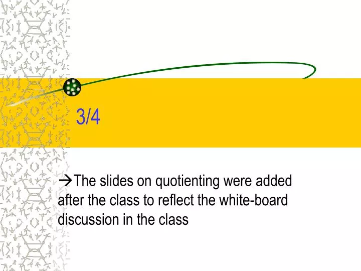
3/4 The slides on quotienting were added after the class to reflect the white-board discussion in the class
Thoughts on Candidate Set semantics for Temporal Planning Doing Temporal Planning Correctly [In search of Complete Position-Constrained Planner] Added after class
Need • Talking about “complete” and “completely optimal” seems to make little sense unless we first define the space over which we want completeness • Qn: What is the space over which candidate set of a temporal plan is defined? • For classical planning, we know it is over “action sequences” • Interestingly, even partial-order planners are essentially aiming for completeness over these action sequences Added after class
Dispatches as candidates • We can define candidate sets in terms of “dispatches” • A dispatch is a set of 3 tuples { <a, sa, ea>} where • a is a ground (durative) action • Sa is the start time for the action a • Ea is the end time for the action a • For fixed duration actions, ea is determined given sa • Completeness, optimality etc should be defined over these dispatches eventually.. Added after class
Quotient spaces • The space of dispatches is “dense” when you have real valued time points • It is more convenient to think of search in terms of quotient spaces defined over the space of dispatches • In fact, it seems necessary that we search in quotient spaces for temporal planning (especially with real-valued time) • Since we want the complexity of planning be somehow related to the number of actions in the plan, and not on their durations(?) • A quotient space essentially involves setting up disjoint equivalence classes over the base space • SNLP’s partial plans actually set up a quotient space over the ground operator sequences (otherwise, the space of partially ordered plans will be much larger than the space of sequences..) • There are multiple ways of setting up quotient spaces over dispatches • You can discuss completeness of any planner w.r.t. any legal quotient space. • But.. Some quotient spaces may be more natural to discuss some planners… Added after class
Start/End point permutations (SEPP) • One quotient space over dispatches is to consider the space of permutations over the start and end points of actions • Specifically, we consider the space of sequences over the alphabet {as ae} over all actions where: • If the sequence contains as, it must contain ae (and vice versa) • as must come before ae in the sequence • If the sequence contains end points of two actions a1 and a2, then their order must not violated durations of the actions • If d(a1)< d(a2), then we can’t have ..a1s…a2s…a2e..a1e.. In the sequence • Note that each element of SEPP space is a representative for a possibly infinite number of dispatches • Completeness over the SEPP space is a necessary condition for completeness over dispatch space Added after class
POP space • The space of partially ordered causal link plans that VHPOP/Zeno search in should be seen as quotienting further over the SEPP space • Similar to the way SNLP plans can be seen as quotienting over the action sequences. Added after class
SAPA-space? • Another way of setting up a quotient space over dispatches is to consider specific dispatches themselves as the prototypes of an equivalence class of dispatches Added after class
Prototype-based quotient spaces • SAPA seems to be easiest to understand in terms of associating a specific dispatch as the representative of a set of dispatches • It then only searches over these dispatches • ..so it will be incomplete if the optimal solution of a problem is not in the space of these canonical dispatches • The basic result of [Cushing et al 2007] can be understood as saying that there is no easy way to set up a finite set of representative dispatches that will be complete for all problems • This, I believe, is the lesson of the failed quest for complete DEP planners • Left-shifted plans as representatives? Added after class
Quotient Space & Navigation?? • Sapa can be understood as • Trying to navigate in a quotient space of left-shifted dispatches • But with an incomplete navigational strategy • Navigation is being effected through epochs • Our inability to find a good epoch-based navigation seems to suggest that there is no natural way to navigate this space? Added after class
Left-shifted plans • Two plans are equivalent if they have the same happening sequence • The canonical representation Added after class
Mid-term Feedback.. • 9 out of 12 gave feedback. I will post them all un-edited. • People generally happy (perhaps embarrassingly happy) with the way the class is going • One person said it is all too overwhelming and the pace and coverage should be reduced significantly • Readings: A mixture of reading before and after. • Homeworks: Majority seem happy that they force them to re-read the paper. There seems to be little support for “more” homework • One person said they should be more challenging and go beyond readings. • Semester project: Majority seem to be getting started; and want to spend time on “their” project rather than homeworks etc. • Interactivity: People think there is enough discussion (I beg to disagree—but I am just an instructor). • One person thought that there should be more discssion--and suggested design of more incentives for discussion • (sort of like the blog discussion requirement)
Qualitative Interval constraints (and algebra) Point constraints (and algebra) Metric constraints Best seen as putting distance ranges over time points Temporal Constraints • Hybrid: allow qualitative and quantitative constraints General temporal constraint reasoning is NP-hard. Tractable subclasses exist. Most temporal constraint formalisms model only binary constraints
Tradeoffs: Progression/Regression/PO Planning for metric/temporal planning • Compared to PO, both progression and regression do a less than complete job of handling concurrency (e.g. slacks may have to be handled through post-processing). • Progression planners have the advantage that the exact amount of a resource is known at any given state. So, complex resource constraints are easier to verify. PO (and to some extent regression), will have to verify this by posting and then verifying resource constraints. • Currently, SAPA (a progression planner) does better than TP4 (a regression planner). Both do oodles better than Zeno/IxTET. However • TP4 could be possibly improved significantly by giving up the insistence on admissible heuristics • Zeno (and IxTET) could benefit by adapting ideas from RePOP.
Salvaging State-space Temporal Planning Interleaving-Space: TEMPO match light • Delay dispatch decisions until afterwards • Choose • Start an action • End an action • Make a scheduling decision • Solve temporal constraints • Temporally Simple • Complete, Optimal • Temporally Expressive • Complete, Optimal fuse fix fix light fix fuse light fix fuse match fix light
Qualitative Temporal Constraints(Allen 83) • y after x • y met-by x • y overlapped-by x • y contains x • y started-by x • y finished-by x • y equals x • x before y • x meets y • x overlaps y • x during y • x starts y • x finishes y • x equals y X Y X Y X Y Y X Y X Y X Y X
Intervals can be handled directly • The 13 in the previous page are primitive relations. The relation between a pair of intervals may well be a disjunction of these primitive ones: • A meets B OR A starts B • There are “transitive” axioms for computing the relations between A and C, given the relations between A and B & B and C • A meets B & B starts C => A starts C • A starts B & B during C => ~ [C before A] • Using these axioms, we can do constraint propagation directly on interval relations; to check for tight relations among any given pair of relations (as well as consistency of a set of relations) • Allen’s Interval Algebra • Intervals can also be handled in terms of their start and end points. This latter is what we will see next.
Qualitative Temporal ConstraintsMaybe Expressed as Inequalities (Vilain, Kautz 86) • x before y X+ < Y- • x meets y X+ = Y- • x overlaps y (Y- < X+) & (X- < Y+) • x during y (Y- < X-) & (X+ < Y+) • x starts y (X- = Y-) & (X+ < Y+) • x finishes y (X- < Y-) & (X+ = Y+) • x equals y (X- = Y-) & (X+ = Y+) Inequalities may be expressed as binary interval relations: X+ - Y- < [-inf, 0]
Metric Constraints • Going to the store takes at least 10 minutes and at most 30 minutes. • 10 < [T+(store) – T-(store)] < 30 • Bread should be eaten within a day of baking. • 0 < [T+(baking) – T-(eating)] < 1 day • Inequalities, X+ < Y- , may be expressed as binary interval relations: • - inf < [X+ - Y-] < 0
Metric Time: Quantitative Temporal Constraint Networks(Dechter, Meiri, Pearl 91) • A set of time points Xi at which events occur. • Unary constraints (a0< Xi < b0 ) or (a1< Xi < b1 ) or . . . • Binary constraints (a0< Xj -Xi < b0 ) or (a1< Xj -Xi < b1 ) or . . . STN (simple temporal network) is a TCN that has no disjunctive constraints (each constraint has one interval) Not n-ary constraints
[30,40] [10,20] [60,inf] 0 1 3 [10,20] 2 4 [20,30] [40,50] [60,70] TCSP Are Visualized UsingDirected Constraint Graphs
TCSPs vs CSPs • TCSP is a subclass of CSPs with some important properties • The domains of the variables are totally ordered • The domains of the variables are continuous • Most queries on TCSPs would involve reasoning over all solutions of a TCSP (e.g. earliest/latest feasible time of a temporal variable) • Since there are potentially an infinite number of solutions to a TCSP, we need to find a way of representing the set of all solutions compactly • Minimal TCSP network is such a representation
TCSP Queries(Dechter, Meiri, Pearl, AIJ91) • Is the TCSP consistent?Planning • What are the feasible times for each Xi? • What are the feasible durations between each Xi and Xj? • What is a consistent set of times?Scheduling • Dispatch • What are the earliest possible times?Scheduling • What are the latest possible times? All of these can be done if we compute the minimal equivalent network
Constraint Tightness & Minimal Networks • A TCSP N1 is considered minimal network if there is no other network N2 that has the same solutions as N1, and has at least one tighter constraint than N1 • Tightness means there are fewer valid composite labels for the variables. This has nothing to do with the “syntactic complexity” of the constraint • A Constraint a[ 1 3]b is tighter than a constraint a[0 10]b • A constraint a[1 1.5][1.6 1.9][1.9 2.3] [2.3 4.8] [5 6]b is tighter than a constraint a[0 10]b • Computation of minimal networks, in general, involves doing two operations: • Intersection over constraints • Composition over constraints • For each path p in the network, connecting a pair of nodes a and b, find the path constraint between a and b (using composition) • Intersect all the constraints between a pair of nodes a and b to find the tightest constraint between a and b • Can lead to “fragmentation of constraints” in the case of disjunctive TCSPs…
Operations on Constraints: Intersection And Composition Compose [10,20] with [30,40][60,inf] to get constraint between 0 and 3
An example where minimal network is different from the original one. [40,60] [10,20] [30,40] [10,20] [30,40] 0 1 3 0 1 3 [0,100] [0,100] To compute the constraint between 0 and 3, we first compose [10,20] and [30,40] to get [40,60] we then intersect [40,60] and [0,100] to get [40,60]
Computing Minimal Networks Using Path Consistency • Minimal networks for TCSPs can be computed by ensuring “path consistency” • For each triple of vertices i,j,k • C(i,k) := C(i,k) .intersection. [C(i,j) .compose. C(j,k)] • For STP’s we are guaranteed to reach fixpoint by the time we visit each constraint once • I.e., outerloop executes only once. • For Disjunctive TCSPs, enforcing path consistency is NP-hard • Shouldn’t be surprising… consistency of disjunctive precedence constraints is NP-hard • “Fragmentation” happens • Approximation schemes possible
Solving Disjunctive TCSPs: Split disjunction • Suppose we have a TCSP, where just one of the constraints is dijunctive: a [1 2][5 6] b • We have two STPs one in which the constraint a[1 2]b is there and the other contains a[5 6]b • Disjunctive TCSP’s can be solved by solving the exponential number of STPs • Minimal network for DTP is the union of minimal networks for the STPs • This is a brute-force method; Exponential number of STPs—many of which have significant overlapping constraints.
20 40 0 1 3 -10 [10,20] -30 [30,40] 0 1 3 -10 20 [10,20] 50 2 4 -40 2 4 -60 [40,50] 70 [60,70] To Query an STN Map to aDistance Graph Gd = < V,Ed > Edge encodes an upper bound on distance to target from source. Xj - Xi£ bij Xi - Xj£ - aij Tij = (aij£ Xj - Xi£ bij)
Conjoined Paths are Computed using All Pairs Shortest Path(e.g., Floyd-Warshall’s algorithm ) 1. for i := 1 to n do dii 0; 2. for i, j := 1 to n do dij aij; 3. for k := 1 to n do 4. for i, j := 1 to n do 5. dij min{dij, dik + dkj}; k i j
20 40 0 1 2 -10 -30 -10 20 50 3 4 -40 -60 70 d-graph Shortest Paths of Gd
STN Minimum Network d-graph STN minimum network
20 40 0 1 2 -10 -30 -10 20 50 3 4 -40 -60 70 Testing Plan Consistency No negative cycles: -5 > TA– TA = 0 d-graph
Latest Solution Node 0 is the reference. 20 40 0 1 2 -10 -30 -10 20 50 3 4 -40 -60 70 d-graph
Earliest Solution Node 0 is the reference. 20 40 0 1 2 -10 -30 -10 20 50 3 4 -40 -60 70 d-graph
Solution: Earliest Times S1 = (-d10, . . . , -dn0) 20 40 0 1 3 -10 -30 -10 20 50 2 4 -40 -60 70
Scheduling:Feasible Values Latest Times • X1 in [10, 20] • X2 in [40, 50] • X3 in [20, 30] • X4 in [60, 70] Earliest Times d-graph
O(N2) Solution by Decomposition • Select value for 1 • 15 • Select value for 2, consistent with 1 • 45 • Select value for 3, consistent with 1 & 2 • 30 d-graph • Select value for 4, consistent with 1,2 & 3
Multi-objective search • Multi-dimensional nature of plan quality in metric temporal planning: • Temporal quality (e.g. makespan, slack—the time when a goal is needed – time when it is achieved.) • Plan cost (e.g. cumulative action cost, resource consumption) • Necessitates multi-objective optimization: • Modeling objective functions • Tracking different quality metrics and heuristic estimation Challenge: There may be inter-dependent relations between different quality metric
Tempe Los Angeles Phoenix Example • Option 1: Tempe Phoenix (Bus) Los Angeles (Airplane) • Less time: 3 hours; More expensive: $200 • Option 2: Tempe Los Angeles (Car) • More time: 12 hours; Less expensive: $50 • Given a deadline constraint (6 hours) Only option 1 is viable • Given a money constraint ($100) Only option 2 is viable
Solution Quality in the presence of multiple objectives • When we have multiple objectives, it is not clear how to define global optimum • E.g. How does <cost:5,Makespan:7> plan compare to <cost:4,Makespan:9>? • Problem: We don’t know what the user’s utility metric is as a function of cost and makespan.
Solution 1: Pareto Sets • Present pareto sets/curves to the user • A pareto set is a set of non-dominated solutions • A solution S1 is dominated by another S2, if S1 is worse than S2 in at least one objective and equal in all or worse in all other objectives. E.g. <C:4,M9> dominated by <C:5;M:9> • A travel agent shouldn’t bother asking whether I would like a flight that starts at 6pm and reaches at 9pm, and cost 100$ or another ones which also leaves at 6 and reaches at 9, but costs 200$. • A pareto set is exhaustive if it contains all non-dominated solutions • Presenting the pareto set allows the users to state their preferences implicitly by choosing what they like rather than by stating them explicitly. • Problem: Exhaustive Pareto sets can be large (exponentially large in many cases). • In practice, travel agents give you non-exhaustive pareto sets, just so you have the illusion of choice • Optimizing with pareto sets changes the nature of the problem—you are looking for multiple rather than a single solution.
Solution 2: Aggregate Utility Metrics • Combine the various objectives into a single utility measure • Eg: w1*cost+w2*make-span • Could model grad students’ preferences; with w1=infinity, w2=0 • Log(cost)+ 5*(Make-span)25 • Could model Bill Gates’ preferences. • How do we assess the form of the utility measure (linear? Nonlinear?) • and how will we get the weights? • Utility elicitation process • Learning problem: Ask tons of questions to the users and learn their utility function to fit their preferences • Can be cast as a sort of learning task (e.g. learn a neual net that is consistent with the examples) • Of course, if you want to learn a true nonlinear preference function, you will need many many more examples, and the training takes much longer. • With aggregate utility metrics, the multi-obj optimization is, in theory, reduces to a single objective optimization problem • *However* if you are trying to good heuristics to direct the search, then since estimators are likely to be available for naturally occurring factors of the solution quality, rather than random combinations there-of, we still have to follow a two step process • Find estimators for each of the factors • Combine the estimates using the utility measure THIS IS WHAT IS DONE IN SAPA
Sketch of how to get cost and time estimates • Planning graph provides “level” estimates • Generalizing planning graph to “temporal planning graph” will allow us to get “time” estimates • For relaxed PG, the generalization is quite simple—just use bi-level representation of the PG, and index each action and literal by the first time point (not level) at which they can be first introduced into the PG • Generalizing planning graph to “cost planning graph” (i.e. propagate cost information over PG) will get us cost estimates • We discussed how to do cost propagation over classical PGs. Costs of literals can be represented as monotonically reducing step functions w.r.t. levels. • To estimate cost and time together we need to generalize classical PG into Temporal and Cost-sensitive PG • Now, the costs of literals will be monotonically reducing step functions w.r.t. time points (rather than level indices) • This is what SAPA does
SAPA approach • Using the Temporal Planning Graph (Smith & Weld) structure to track the time-sensitive cost function: • Estimation of the earliest time (makespan) to achieve all goals. • Estimation of the lowest cost to achieve goals • Estimation of the cost to achieve goals given the specific makespan value. • Using this information to calculate the heuristic value for the objective function involving both time and cost • Involves propagating cost over planning graphs..
Heuristics in Sapa are derived from the Graphplan-style bi-level relaxed temporal planning graph (RTPG) Progression; so constructed anew for each state..
A B Person Airplane Person t=0 tg Load(P,A) Unload(P,A) Fly(A,B) Fly(B,A) Unload(P,B) Init Goal Deadline Note: Bi-level rep; we don’t actually stack actions multiple times in PG—we just keep track the first time the action entered Relaxed Temporal Planning Graph RTPG is modeled as a time-stamped plan! (but Q only has +ve events) • Relaxed Action: • No delete effects • May be okay given progression planning • No resource consumption • Will adjust later • while(true) • forallAadvance-time applicable in S • S = Apply(A,S) • Involves changing P,,Q,t • {Update Q only with positive • effects; and only when there is no other earlier event giving that effect} • ifSG then Terminate{solution} • S’ = Apply(advance-time,S) • if (pi,ti) G such that • ti < Time(S’) and piS then • Terminate{non-solution} • elseS = S’ • end while; Deadline goals