LECTURE 28: HIERARCHICAL CLUSTERING

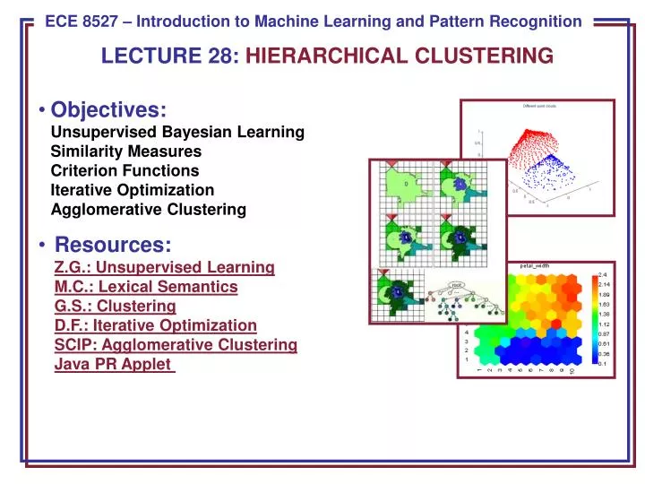
1. LECTURE 28: HIERARCHICAL CLUSTERING • Objectives:Unsupervised Bayesian LearningSimilarity MeasuresCriterion FunctionsIterative OptimizationAgglomerative Clustering • Resources:Z.G.: Unsupervised LearningM.C.: Lexical SemanticsG.S.: ClusteringD.F.: Iterative OptimizationSCIP: Agglomerative ClusteringJava PR Applet

2. The Bayes Classifier • Maximum likelihood methods assume the parameter vector is unknown but do not assume its values are random. Prior knowledge of possible parameter values can be used to initialize iterative learning procedures. • The Bayesian approach to unsupervised learning assumes θis a random variable with known prior distribution p(θ), and uses the training samples to compute the posterior density p(θ|D). • We assume: • The number of classes, c, is known. • The prior probabilities, P(ωj), for each class are known, j = 1, …, c. • The forms of the class-conditional probability densities, p(x|ωj,θj) are known, j = 1, …, c, but the full parameter vector θ= (θ1, …,θc)t is unknown. • Part of our knowledge about θis contained in a set D of n samples x1, …, xn drawn independently from: • We can write the posterior for the classassignment as a function of the featurevector and samples:

3. The Bayes Classifier (cont.) • Because the state of nature, ωi, is independent of the previously drawn samples, P(ωi|D) = P(ωi), we obtain: • We can introduce a dependence on the parameter vector, θ: • Selection of x is independent of the samples: • Because the class assignment when x is selected tells us nothing about the distribution of θ: • We can now write a simplified expression for : • Our best estimate of is obtained by averaging over θi. The accuracy of this estimate depends on our ability to estimate .

4. Learning The Parameter Vector • Using Bayes formula we can write an expression for : • We can write an expression for using our independence assumption (see slide 11, lecture no. 7): • If is uniform over the region where peaks, then (from Bayes rule), peaks at the same location. If the only significant peak occurs atand if the peak is very sharp, then: • and • This is our justification for using the maximum likelihood estimate, , as if it were the true value of θin designing the Bayes classifier. • In the limit of large amounts of data, the Bayes and ML estimates will be very close.

5. Additional Considerations • If p(θ)has been obtained by supervised learning from a large set of labeled samples, it will be far from uniform and it will have a dominant influence on p(θ|Dn) when n is small. • Each sample sharpens p(θ|Dn). In the limit it will converge to a Dirac delta function centered at the true value of θ. • Thus, even though we don’t know the categories of the samples, identifiabiliy assures us that we can learn the unknown parameter θ. • Unsupervised learning of parameters is very similar to supervised learning. • One significant difference: with supervised learning the lack of identifiability means that instead of obtaining a unique parameter vector, we obtain an equivalent class of parameter vectors. • For unsupervised training, a lack of identifiability means that even thoughp(θ|Dn) might converge to p(x), p(x|θi,Dn) will not in general converge to p(x|θi). In such cases a few labeled training samples can have a big impact on your ability to decompose the mixture distribution into its components.

6. Decision-Directed Approximation • Because the difference between supervised and unsupervised learning is the presence of labels, it is natural to propose the following: • Use prior information to train a classifier. • Labelnew data with this classifier. • Use the new labeled samples to train a new (supervised) classifier. • This approach is known as the decision-directed approach to unsupervised learning. • Obvious dangers include: • If the initial classifier is not reasonably good, the process can diverge. • The tails of the distribution tend not to be modeled well this way, which results in significant overlap between the component densities. • In practice, this approach works well because it is easy to leverage previous work for the initial classifier. • Also, it is less computationally expensive than the pure Bayesian unsupervised learning approach.

7. Similarity Measures • How should we measure similarity between samples? • How should we evaluate a partitioning of a set of samples into clusters? • Theanswer to both requires an ability to measure similarity in a way that is meaningful to the problem. For example, in comparing two spectra of a signal for an audio application, we would hope a spectral distance measure compares closely to human perception. We often refer to this as a “perceptually-meaningful” distance measure, and this concept is more general than audio. • Principal components can also be used to achieve invariance prior to clustering through normalization. • One broad class of metrics is the Minkowski metric: • Another nonmetric approach measures the angle between two vectors:

8. Criterion Functions For Clustering • Sum of squared errors: • Minimum variance criteria: • Scatter Matrices (e.g., ST=SW+SB) • Trace Criterion: • Determinant Criterion: • Invariant Criteria (eigenvalues are invariant under linear transformations):

9. Iterative Optimization • Because the sample set is finite, clustering can be viewed as a problem solved by exhaustive enumeration. However the computational complexity of this approach is prohibitive (cn/c!). • However, we can apply an iterative hill-climbing procedure: • Generate an initial clustering. • Randomly select a point. • Test whether assigning it to another cluster will reduce the error(e.g., mean squared error); move to the appropriate cluster. • Iterate until no further reassignments are made. • Note that efficient methods exist for updating the cluster means and overall error because we only need to consider the contribution from this one point. • This can be considered a sequential form of the k-Means algorithm. • Obvious drawbacks include the potential to get stuck in local minima. One way around this is to use a hybrid approach (e.g., alternate between this and standard k-Means algorithm).

10. Hierarchical Clustering • We seek a clustering technique that imposes a hierarchical structure on the data, much like a decision tree. • Let us consider a sequence of partitions of n samples into c clusters. • In the first partition, there are n clusters, each with one sample. • In the next partition, there are n-1 clusters. At level k, there are n-k+1 clusters. • If two samples in a cluster at level k remain in the same cluster for higher levels, the clustering technique is referred to as hierarchical clustering. • This graphical representation ofthis process shown to the rightis referred to as a dendrogram. • Similarity values can be used tohelp determine whether groupingsare natural or forced (e.g., if thevalues are comparable acrossa level, then there is probablyno strong argument for any particularclustering of the data. • Venn diagrams can also be used to depict relationships between clusters.

11. Agglomerative Clustering • Hierarchical clustering is very popular as an unsupervised clustering method. • Two distinct approaches: (1) agglomerative – bottom up, and (2) divisive (top down). The well-known Linde-Buzo-Gray (LBG) algorithm is divisive. • Agglomerative clustering typically requires less computation to go from one level to the next. • Divisive clustering requires less computation if the goal is a small number of clusters (e.g., c/n << 1). • Agglomerative hierarchical clustering: • Begin: initialize • Do • Find nearest clusters, Di and Dj • Merge Di and Dj • Until • Return c clusters • End • If we continue this process until c = 1, we produce the dendrogram shown above.

12. Agglomerative Clustering (cont.) • It is common to use minimum variance type distance measures: • When dmin is used, this is referred to as a nearest-neighbor cluster algorithm. • Computational complexity: • Need to calculate n(n-1)interpoint distances, each is O(d), and store them in a table, which is O(n2) in memory. • Finding the minimum distance pair requires stepping through the entire list. • Overall complexity: O(n(n-1)(d+1)) = O(n2d). In general, O(cn2d) where n >> c. • But there are faster implementations of these approaches. Memory becomes a major bottleneck for large data sets. Disk caching becomes important.

13. Spanning Trees • Single-linkage algorithm: The clustering algorithm is terminated when the distance between the nearest clusters exceeds an arbitrary threshold. • Spanning Tree: A tree with any path from one node to any other node, but no cycles or closed loops. • Minimum Spanning Tree: A spanning tree with a minimal number of edges, which you can obtain by using a minimum distance criterion. • Stepwise Optimal Hierarchical Clustering: • Begin: initialize • Do • Find clusters whose merger changes the criterion least, say Di and Dj • Merge Di and Dj • Until • Return c clusters • Clustering algorithms often use a confusion matrix measuring the dissimilarity of the data (induced metrics).

14. Demonstrations

15. Summary • Reviewed the Bayes classifier. • Revisited unsupervised Bayesian learning using a recursive approach. • Compared ML and Bayes estimates. • Compared supervised vs. unsupervised learning. • Discussed computational considerations. • Discussed hybrid methods (decision-directed) approaches to learning. • Reviewed similarity measures and criterion functions. • Discussed iterative optimization techniques. • Introduced hierarchical clustering methods (agglomerative vs. divisive). • Introduce the concept of spanning trees.