Download
1 / 31
320 likes | 527 Vues
M. Weigelt, W. Keller. Grace GRAVITY FIELD SOLUTIONS USING THE DIFFERENTIAL GRAVIMETRY APPROACH. Continental Hydrology. Geodesy. Oceano - graphy. Solid Earth. Glacio - logy. Earth core. Tides. Atmosphere. Geophysical implications of the gravity field. Geoid.

E N D
M. Weigelt, W. Keller Grace GRAVITY FIELD SOLUTIONS USING THE DIFFERENTIAL GRAVIMETRY APPROACH
Continental Hydrology Geodesy Oceano- graphy Solid Earth Glacio- logy Earth core Tides Atmosphere Geophysicalimplicationsofthegravityfield Geoid
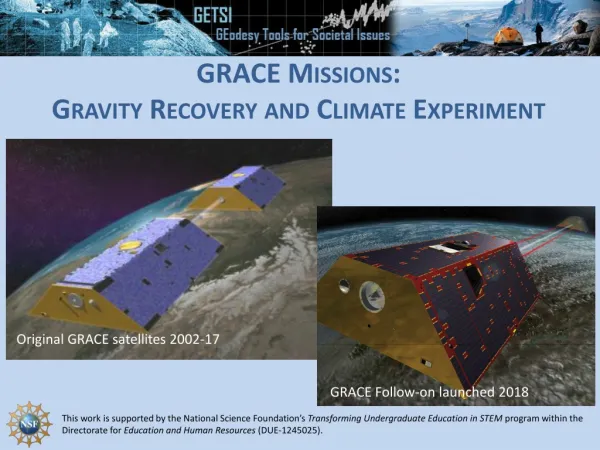
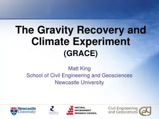
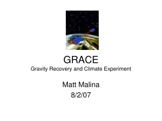
Observation system GRACE = Gravity Recovery and Climate Experiment • Initial orbit height: ~ 485 km • Inclination: ~ 89° • Key technologies: • GPS receiver • Accelerometer • K-Band Ranging System • Observed quantity: • range • range rate CSR, UTexas
Gravity field modelling with gravitational constant times mass of the Earth radius of the Earth spherical coordinates of the calculation point Legendre function degree, order (unknown) spherical harmonic coefficients
Spectral representations Degree RMS Spherical harmonic spectrum
Outline • GRACE geometry • Solution strategies • Variational equations • Differential gravimetry approach • What about the Next-Generation-GRACE?
Geometry of the GRACE system B A Differentiation Rummel et al. 1978 Integration
Solution strategies Variational equations In-situ observations Energy Integral (Han 2003, Ramillien et al. 2010) Classical (Reigber 1989, Tapley 2004) Celestial mechanics approach • (Beutler et al. 2010, Jäggi 2007) Differential gravimetry (Liu 2010) LoS Gradiometry (Keller and Sharifi 2005) Short-arc method (Mayer-Gürr 2006) … … Numericalintegration Analyticalintegration
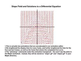
Equation of motion Basic equation: Newton’s equation of motion where are all gravitational and non-gravitational disturbing forces In the general case: ordinary second order non-linear differential equation Double integration yields:
Linearization For the solution, linearization using a Taylor expansion is necessary: • Types of partial derivatives: • initial position • initial velocity • residual gravity field coefficients • additional parameter Homogeneous solution Inhomogeneous solution …
Homogeneous solution Homogeneous solution needs the partial derivatives: Derivation byintegrationofthevariationalequation Double integration !
Inhomogeneous solution (one variant) Solution of the inhomogeneous part by the method of the variation of the constant (Beutler 2006): with being the columns of the matrix of the variational equation of the homogeneous solution at each epoch. Estimation of by solving the equation system at each epoch:
Application to GRACE In case of GRACE, the observables are range and range rate: Chain rule needs to be applied:
Limitations • additional parameters • compensate errors in the initial conditions • counteract accumulation of errors • outlier detection difficult • limited application to local areas • high computational effort • difficult estimation of corrections to the initial conditions in case of GRACE (twice the number of unknowns, relative observation)
In-situ observations: Differential gravimetry approach
Instantaneous relative reference frame Position Velocity
In-situ observation Range observables: Multiplication with unit vectors: GRACE
Relative motion between two epochs absolute motion neglected! GPS Epoch 1 K-Band Epoch 2
Limitation Combination of highly precise K-Band observations with comparably low accurate GPS relative velocity
Residual quantities estimated orbit GPS-observations true orbit Orbit fitting using the homogeneous solution of the variational equation with a known a priori gravity field Avoiding the estimation of empirical parameters by using short arcs
Residual quantities ratio≈ 1:2 ratio≈ 25:1
Next generation GRACE M. Dehne, Quest New type of intersatellite distance measurement based on laser interferometry Noise reduction by a factor 10 expected
Variational equations for velocity term Reduction to residual quantity insufficient Modeling the velocity term by variational equations: Application of the method of the variations of the constants
Results • Only minor improvements by incorporating the estimation of corrections to the spherical harmonic coefficients due to the velocity term • Limiting factor is the orbit fit to the GPS positions • additional estimation of corrections to the initial conditions necessary
Summary The primary observables of the GRACE system (range & range rate) are connected to gravity field quantities through variational equations (numerical integration) or through in-situ observations (analytical integration). Variational equations pose a high computational effort. In-situ observations demand the combination of K-band and GPS information. Next generation GRACE instruments pose a challenge to existing solution strategies.