Download
1 / 40
400 likes | 495 Vues
Constrained Bayes Estimates of Random Effects when Data are Subject to a Limit of Detection. Reneé H. Moore Department of Biostatistics and Epidemiology University of Pennsylvania Robert H. Lyles, Amita K. Manatunga , Kirk A. Easley

E N D
Constrained Bayes Estimates of Random Effects when Data are Subject to a Limit of Detection Reneé H. Moore Department of Biostatistics and Epidemiology University of Pennsylvania Robert H. Lyles, Amita K. Manatunga, Kirk A. Easley Department of Biostatistics and Bioinformatics Emory University
Outline • Motivating Example • Background • Review the Mixed Linear Model • Bayes predictor • Censoring under the Mixed Model • CB Predictors • Application of Methodology for CB adjusted for LOD • Motivating Example • Simulation Studies
P2C2 HIV Infection Study: Is this Child’s HIV Infection at Greater Risk of Rapid Progression? • 1990-1993 HIV transmitted from mother to child in utero • Children in this dataset enrolled at birth or by 28 days of life • HIV RNA Data at 3-6mos through 5 years of age • Rapid Progression is defined as the occurrence of AIDS (Class C) or death before 18 months of age • One goal of the study was to identify children with RP of disease because they may benefit from early and intense antiretroviral therapy
Is this Child’s HIV Infection at Greater Risk of Rapid Progression? • One Indicator: high initial and/or steeply increasing HIV RNA levels over time • Limitation: HIV RNA below a certain threshold not quantifiable • Given non-detects, how do we predict each child’s HIV RNA intercept and slope? • Given non-detects, how do we predict each child’s HIV RNA level at a meaningful time point associated with RP?
The Mixed Linear Model Y: N by 1 outcome variable X: known N by p fixed effects design matrix : p by 1 vector of fixed effects Z: known N by q random effects design matrix u: q by 1 vector of random effects e: N by 1 vector of random error terms
The Mixed Linear Model Assumptions: E(u)= 0 and E(e)= 0
BP (best predictor, Searle et.al. 1992): - minimizes - invariant to the choice of A, any pos. symmetric matrix - holds regardless of joint distribution of (u, Y) - unbiased, i.e. - linear in Y “Bayes Predictor” E(u|Y)
Censoring under the mixed model *common feature of HIV data is that some values fall below a LOD • Ad hoc approach: substitute the LOD or a fraction of it for all values below the limit (Hornung and Reed, 1990) • Other Approaches: • - Likelihood using the EM algorithm (Pettitt 1986, Hughes 1991) • - Bayesian Methods (Carriquiry 1987) • - Likelihood based approach using algortihms (Jacgmin-Gadda et.al. 2000) • Lyles et. al. (2000) maximize an integrated joint log-likelihood directly to handle informative drop-out and left censoring
Left-censoring under the mixed model Lyles et.al. (2000) work under framework of (i = 1, … , k ; j=1, …, ni) To get estimates of = - ni1 detectable measurements: f(Yij|ai,bi) - ni - ni1non-detectable measurements: FY(d|ai ,bi)
E(u|Y)can’t be calculated in practice! Why? - knowledge of all parameters in the joint distribution of (u,Y) What do we do? - develop predictors based on their theoretical properties for known parameters - evaluate effect of estimating unknown parameters via simulation studies
Bayes Predictor (posterior mean) E(u|Y) • minimizes MSEP s.t. tends to overshrink individual ui toward u • - Prediction Properties (bias, MSEP) deteriorate for individuals whose random effects put them in tails of distribution • Motivated research for alternatives to Bayes • Limited translation rules (Efron and Morris, 1971) • Constrained Bayes
Bayes with LOD Lyles et al. (2000), using the MLEs from L( ;Y),
Censoring under the mixed model None of the references cited for dealing with left-censored longitudinal or repeated measures data considered alternatives to the Bayes predictors for random effects We Do!
Constrained Bayes Estimation • Louis (1984) • Expectation of sample variance of Bayes estimates is only a fraction of expected variance of unobserved parameters derived from the prior • Shrinkage of the Bayes estimate • Reduces shrinkage by matching first two moments of estimates with corresp. moments from posterior histogram of k normal means
Constrained Bayes Estimation • Ghosh (1992): “recipe” to generalize Louis’ modified Bayes predictor for use with any distribution • Lyles and Xu (1999): match predictor’s mean and variance with prior mean and variance of random effect
Constrained Bayes Estimation Ghosh (1992) where
Constrained Bayes Estimation minimizes MSEP = within the class of predictors of satisfies (1) but NOT (2) Ghosh (1992) s.t. (1) posterior mean matches sample mean (2) posterior variance matches sample variance Adjust Recall: Bayes Con. Bayes
Constrained Bayes (CB) Estimation CB Predictors have been shown to reduce the shrinkage of the Bayes estimate in an appealing way BUT none had been adapted to account for censored data We Do! Moore, Lyles, Manatunga (2010). Empirical constrained Bayes predictors accounting for non-detects among repeated Measures. Statistics in Medicine.
CB Predictors with LOD • Lyles (2000): adjusted Bayes estimate to accommodate data subject to a LOD but did not consider CB • Moore (2010): combine Lyles (2000) BayesLOD and Ghosh (1992) CB CBLOD
(i = 1, … , k ; j=1, …, ni) Intercept: Slope: • Yij : Observed HIV RNA measurement at jth time point (tij)for ith child • ai : ith child’s random intercept deviation • bi: ith child’s random slope deviation Random Intercept-Slope Model
Under random intercept-slope model, Lyles et.al. (2000) get MLEs of = • ni1 detectable measurements: f(Yij|ai,bi) • ni - ni1non-detectable measurements: FY(d|ai,bi) • d= limit of detection (LOD)
minimizes MSEP s.t. posterior mean matches sample mean strongly shrinks predicted βi toward β or αi toward α • Prediction properties (bias, MSEP) deteriorate for individuals whose random effects put them in the tail of the distribution Bayes Predictor for LOD
(i = 1, … , k ; j=1, …, ni) CB Predictions of αiand βi
Comparing Constrained Bayes EstimatesParameter Estimates Based on 2 Methods: Ad Hoc Imputation & Adjust Likelihood for LOD
Example Simulation Study Table IV. (Moore et al. Statistics in Medicine, 2010)
Is this Infant’s HIV Infection at Greater Risk of Rapid Progression? • Given non-detects, how do we predict each patient’s HIV RNA intercept and slope? • Viable option now available • Given non-detects, how do we predict each patient’s HIV RNA level at a meaningful time point? • Extending our Stat in Med 2010 work
Is this Child’s HIV Infection at Greater Risk of Rapid Progression? P2C2 HIV Data (Chinen, J., Easley, K. et.al., J. Allergy Clin. Immunol. 2001) • 343 HIV RNA measurements from 59 kids (range: 2-11, median=6) • detection limit= 2.6 =log(400 copies/mL) • 6% (21 /343) of measurements < LOD • 19% (11 /59) kids have at least one meas. < LOD • 59 unique times (t) reached Class A HIV* Goal: Predict Yit: HIV RNA level at time reached Class A
Prediction of Yit = αi+ t βi • Recall: Yij= (α + ai) + (β + bi)tij + εij • Goal of Predictor is to Match • Compare and
Prediction of Yit = αi + t βi • Our previous CB predictors set out to match but did not enforce constraint • We develop a CB predictor for the scalar R.V. Yit
Objective 1: Prediction of Yit = αi + t βi What is new in adapting this extension of Ghosh’s CB? • calculated for all k subjects at each unique t
The 59 Individual Predictors ofYitat each Child’s Unique t • Bayes • CB
Simulation Study for Yit • Parameter Assumptions: • 1500 subjects, each with five HIV RNA values taken every six months for 2 years • 15% (1,089 /7,500) values < LOD = 2.8 • 8 times (t) of interest = (0.03, 0.16, 0.36, 0.66, 0.85, 1.17, 1.32, 1.60)
Sample Variance Sample Mean Sample Variance Simulation Study for Yit
Bayes (closed circles) and CB (open circles) estimates of 80 simulated patients. The line plotted is . . Simulation Study for Yit .
Summary • Proposed LOD-adjusted CB predictors - Intercepts and Slopes - R.V. (Yit) at a meaningful time point Relative to ad hoc and Bayes predictors: “CBs Attenuate the Shrinkage” Better Match True Distribution of Random Effects