Download
1 / 25
250 likes | 393 Vues
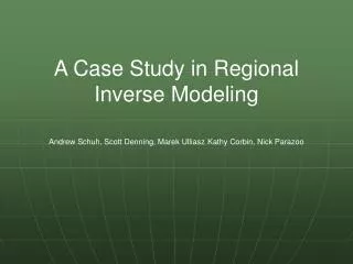
A Case Study in Regional Inverse Modeling. Andrew Schuh, Scott Denning, Marek Ulliasz Kathy Corbin, Nick Parazoo. The Question: How is NEE distributed across domain in both time and space and how to capture at different scales. Deterministic Biosphere and Transport Models.

E N D
A Case Study in Regional Inverse Modeling Andrew Schuh, Scott Denning, Marek UlliaszKathy Corbin, Nick Parazoo
The Question:How is NEE distributed across domain in both time and space and how to capture at different scales
Deterministic Biosphere and Transport Models • SiB2.5 is used for biosphere model. MODIS fPAR and LAI products are used to drive SiB2.5. • coupled to RAMS 5.0, meteorology forced with Eta 40km reanalysis data • 150 x 100 40km grid over North America for the • time period: 5/1/2004 through 8/31/2004.
Inversion Methods Available • Bayesian Synthesis Inversion • For many problems the quickest and easiest method • at core of many inversion methodologies • However, computational concerns arise if the dimensions of the problem get too large
Inversion Methods Available • Kalman filtering techniques • Reduces the effect of the time dimension of inversion problem by putting in state space framework and updating model in time. • EnKF further reduces dimensional constraints by effectively working with a sampled spatial covariance structure. EnKF has also been shown to have some desirable properties for non-linear models.
Inversion Methods Available • What about dealing with the spatial structure of the problem in a hierarchical way? • Inversion can take advantage of implicit spatial structure inherent in many spatial characterizations, like ecoregions • Covariance properties are propagated through a hierarchical covariance structure, independent within levels, thus reducing dimensionality of the covariance
Hierarchical Model (Model Domain) βI=1 βI=2 LEVEL 2 ECOREGIONS LEVEL 3 ECOREGIONS βI=3 βI=4 βI=4,II=1 βI=4,II=2 LEVEL 1 ECOREGIONS βI=4,II=1,III=1 βI=4,II=1,III=2 βI,=4,II=3 βI=4,II=4 βI=4,II=1,III=3 βI=4,II=1,III=4
Example • A backward in time lagrangian particle model (LPDM) was used in conjunction with a 4 month SiB2.5Rams simulation to produce “influence functions” for assimilation and respiration for 34 towers. • Four afternoon observations each day for May 10, 2004 - August 31, 2004 were used at each of the 34 towers.
Work to do • Currently inverting on this structure with 2004 data from 8 towers • Explore effects of stepping inversion through time, in state space way. • Subnesting down to SiBRAMS grid size in areas with high density of measurements
What about boundary conditions? • Initial SiBRAMS run had constant carbon dioxide for boundary conditions. • What effect might this have on the simulation? • How might corrections be made to these boundary inflow terms?
Boundary conditions • boundary conditions can be very important to regional scale inversion • The boundaries also represent a large spatial area, possibly contributing many unknowns to an often already under constrained problem • Principal Components for boundary? These provide “directions” of maximal variability (in time) in the boundary conditions.
1st PC Reconstruction of Boundary Influences Sequence of Afternoon Observations for 5/1/2004 - 8/31/04(WLEF,ARM,Harvard,BERMS, BOREAS, Fraserdale, KWKT, Howland)
Boundary conditions • The first principal component generally represents about 75% - 85% of the total variation over time with the second representing another 3% - 6%. • The PCs appear to load nicely, particularly zonally. • Appears to be a promising dimension reduction • An obvious assumption here is that PCTM captures the major modes of variability. Deficiencies in the transport mechanisms of PCTM can not be expected to be captured via these PCs.
Work to do • Investigating real errors in boundary condition estimates • Exploring relationship between time period of inversion and boundary predictor • Comparing against other simple correction schemes, 2 box vertical, etc