Chapter 10: Speed, Travel Time, and Delay Studies

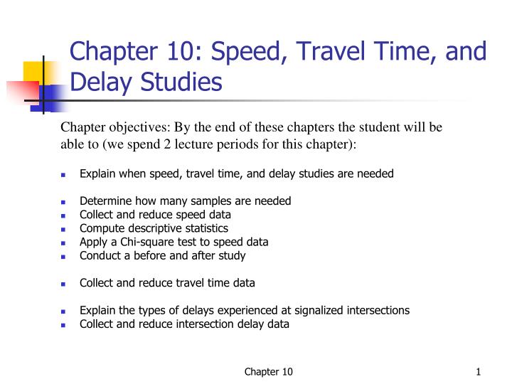
1. Chapter 10: Speed, Travel Time, and Delay Studies • Explain when speed, travel time, and delay studies are needed • Determine how many samples are needed • Collect and reduce speed data • Compute descriptive statistics • Apply a Chi-square test to speed data • Conduct a before and after study • Collect and reduce travel time data • Explain the types of delays experienced at signalized intersections • Collect and reduce intersection delay data Chapter objectives: By the end of these chapters the student will be able to (we spend 2 lecture periods for this chapter): Chapter 10

2. 10.1 Introduction They are used to evaluate the performance of a traffic facility, like arterials and signalized intersections. “Speed” here is a so-called a spot speed measured by a radar gun, etc., at a point in the facility. If you determine travel time and compute speed for a relatively long section, then it is a space speed. Chapter 10

3. 10.2.2. Uses of spot speed data Spot speed studies are conducted to estimate the distribution of speeds of vehicles in a stream of traffic at a particular location on a highway. • Used for: • Establish the effectiveness of new or existing speed limits and/or enforcement practices • Establish trends to assess the effectiveness of national policy on speed limits and enforcement • Specific design applications (like sight distance) • Specific control applications (yellow/all red timing – the size of dilemma zone depends on speed) • Investigation of high-accident locations at which speed is suspected to be a causative factor Chapter 10

4. f(ui – u)2 s = N - 1 10.2.1 and 10.2.4 Speed definitions of interest u = uj/N Chapter 10

5. 85% 50% See table 10.1. Chapter 10

6. 10.2 Spot Speed Studies Once data are collected, the first thing you do is to compute several descriptive statistics to get some ideas about the distribution of the speed data. (Note that many statistical analyses used in traffic engineering assume data are normally distributed.  So, the goal is to check whether they are really normally distributed.) • Typical descriptive statistics are: • Average speed • Variance and standard deviation • Median speed • Modal speed (or Modal speed range  Needs a histogram) • The ith-percentile spot speed • Pace  Usually a 10-mph interval that has the greatest number of observations. (These concepts appeared in chapter 7.) Chapter 10

7. Speed Sample Size For percentile speed comparisons This table is for two-sided tests. K = z-score Chapter 10

8. Location, time of day, and duration… The objective and scope of the study dictate these. At least 1 hour or at least 30 data (if you want to assume normal distribution, but usually you should collect at minimum 100 speeds.) Chapter 10

9. 10.2.3 Analysis of Spot Speed Chapter 10

10. Chapter 10

11. Pace Chapter 10

12. Chi-square (2-) test(So called “goodness-of-fit” test), p.143 Example: Distribution of height data in Table 7-9. H0:The underlying distribution is uniform. H1: The underlying distribution is NOT uniform. The authors intentionally used the uniform distribution to make the computation simple. We will test a normal distribution in class using Excel.

13. Steps of Chi-square (2-) test • Define categories or ranges (or bins) and assign data to the categories and find ni = the number of observations in each category i. (At least 5 bins and each should have at least 5 observations.) • Compute the expected number of samples for each category (theoretical frequency), using the assumed distribution. Define fi = the number of samples for each category i. • Compute the quantity:

14. Steps of Chi-square (2-) test (cont) • 2 is chi-square distributed (see Table 7-11, p.145). If this value is low if our hypothesis is correct. Usually we use  = 0.05 (5% significance level or 95% confidence level). When you look up the table, the degree of freedom is f = N – 1 – g where g is the number of parameters we use in the assumed distribution. For normal distribution g = 2 because we use µ and  to describe the shape of normal distribution. • If the computed 2 value is smaller than the critical c2 value, we accept H0. Why g = 2 for normal distribution? See Eq. 7-7 in p.125.

15. What’s the Chi-square (2-) test testing? You need to know how to pull out values from the assumed distribution to create the expected histogram. Assumed distribution Expected distribution (or histogram) Actual histogram Chi-square (2-) test tests this relationship.

16. p.207 Before and After Spot Speed Studies • Two questions that must be answered: • Is the observed reduction in average speeds real? – checked by comparison of the means test (Was there any statistical difference?) – Use the simple z- or t-test depending on the number of samples and select a one-way or two-way test depending on the hypothesis you want to test.) • Is the observed reduction in average speeds the intended 5 mph (or whatever the value expected) – checked by the confidence interval to see if the targeted speed is within the confidence interval of the after speed value (Was the goal achieved? Use only the results of the “after” distribution. This is done by two-way test. Why?) Review 7.8.2. Chapter 10

17. Part 2: Was the target speed achieved? Example in p.209 Part 1: One-way (zc = 1.645) or two-way test (zc = 1.96)? Chapter 10

18. 10.3 Travel-time (travel delay) studies * Determines the amount of time required to travel from one point to another on a given route. Often, information may also be collected on the locations, durations, and causes of delays • Indicate the level of service • Identify problem locations Chapter 10

19. Applications of travel time and delay data(p.211) Many uses of travel time data Efficiency check Collection of rating data Problem location identification Model calibration Evaluation of performance before and after improvement Collect data for economic analysis (user costs) (like ramp metering vs. no metering) Chapter 10

20. 10.3.1 Field study techniques Methods requiring a test vehicle: Chapter 10

21. License-plate method NG for a grid network – too many routes Use of ETC for freeways Methods not requiring a test vehicle: Bluetooth technology Chapter 10

22. Chapter 10

23. 10.3.2 TT along an arterial: An example of the statistics of TT • (Usually) the distribution of running times is considered normal, but the distribution of travel time is not (because stopped delays at the intersections may follow a completely different distribution). • Example: Mean running time = 196 sec, the SD of the running time = 15 sec. See the discussion of speeds obtained by these values in page 214. (This problem is talking about running time only.) Note that this discussion has nothing to do with Table 10.4. Chapter 10

24. What about travel times?, p.214, Fig 10.3 Mean RT = 196 sec Mean TT = 218.5 sec SD of TT = 38.3 sec This example has 20 travel-time data. This graph does not look normal because travel time = running time + stopped delay. Running times distribute like a normal distribution. Delay distribution is not as shown in this table. Chapter 10

25. Fig 10.3 Adding the average delay time to the average running time (196 sec). 10.3.3 Skipped. Chapter 10

26. 10.3.4 Travel-time displays • Use of travel time data: • A travel time contour as an example Relation between ideal flow and actual flow Chapter 10

27. 10.4 Intersection Delay Studies Travel time and delay studies take delays at signalized intersections but such samples (observations) are not adequate to evaluate the delay at a particular signalized intersection.  Conduct an intersection delay study. Measure of effectiveness  Delay (Current HCM2010 uses the “average control delay”, but previous one (before HCM 2000) used the “average stopped delay.” The average control delay: the total delay at an intersection caused by a control device, including both time-in-queue delay plus delays due to acceleration and deceleration (We will discuss these delays later in the semester). Chapter 10

28. Delay Types • Stopped-time delay - completely stopped • Approach delay – Adds delays by acceleration and deceleration to stopped-time delay • Time-in-queue delay = (time to cross the stop line) – (time when joined a queue), meaning in between the vehicle is in stop-and-go state. (Remember how queued vehicles are released.) • Control delay = (time-in-queue delay) + (accel/decel delay) • Travel-time delay = (actual travel time) – (desired travel time) (Just an intro. We will study these later.) Chapter 10

29. 4 assumptions made for control delay field measurements (p.219) • Meant for undersaturated flow conditions (max queue is about 20 to 25 vehicles. • Does not directly measure acceleration-deceleration delay. Use an adjustment factor to estimate this component • Uses an adjustment to correct for errors that are likely to occur in the sampling process • Must make an estimate of free-flow speed before beginning a detailed survey (drive through the approach before collecting data). Need to determine accel/decel delay adjustment: see Tab 10.6. Start at the beginning of the red phase of the subject lane group. No overflow queue should exist from the previous green phase (ideally). Chapter 10

30. HCM 2010: Intersection delay study method (by lane group) Task 1: Observer 1 keeps track of the end of standing queues for each cycle by observing the last vehicle in each lane that stops due to the signal. This includes vehicles that arrive on green but stop or approach within one car length of queued vehicles that have not yet started to move. See Fig. 10-9 for a sample survey form and Tab 10-7 for a sample data. Observer 1 Observer 2 Task 2: Record the number of vehicles in queue on the field sheet (at the end of the interval). Vehicles in queue are those that are included in the queue of stopping vehicles (as defined in Task 1) and have not yet exited the intersection. Count arriving vehicles & the number of vehicles that stops once or more. Stopping vehicles are counted only once, regardless the number of times they stop. The count interval is typically between 10 sec and 20 sec. It should be an integral divisor of the cycle length. Task 3:At the end the survey period, vehicle-in-queue counts continue until all vehicles that entered the queue during the survey period have exited the intersections. (Observer 1) Chapter 10

31. Delay data collection form (fig 10.9 & Handout) Figure 10.9 Chapter 10

32. Average time-in-queue estimation (10-15) Chapter 10

33. Adjustments for accel/decel delay (10-16) (10-18) Table 10.6: (10-17) Table 10.6: Chapter 10

34. (10-17) and (10-18) veh/ln/cycle Chapter 10

35. 10 second interval seems to be the best compromise according to my study with Jay Walker. Chapter 10