Download
1 / 16
160 likes | 236 Vues
Review. Find the mean square ( MS ) based on these two samples. 26.1 32.7 43.6 65.3 792.7. +14 +14. M A = 14. Flood. -27 -41 -41. M B = -36.3. Review. The mean square is MS = 43.6. Now find the standard error, 6.0 8.5 19.5 36.3 56.0. +14 +14. M A = 14. Flood. -27

E N D
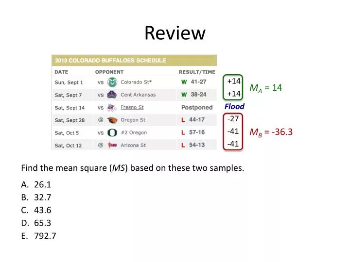
Review Find the mean square (MS) based on these two samples. • 26.1 • 32.7 • 43.6 • 65.3 • 792.7 +14 +14 MA = 14 Flood -27 -41 -41 MB = -36.3
Review The mean square is MS = 43.6. Now find the standard error, • 6.0 • 8.5 • 19.5 • 36.3 • 56.0 +14 +14 MA = 14 Flood -27 -41 -41 MB = -36.3
Review The standard error is . Now calculate t. • 3.7 • 8.4 • 133.8 • 301.8 +14 +14 MA = 14 Flood -27 -41 -41 MB = -36.3
Effect Size 10/17
Effect Size • If there's an effect, how big is it? • How different is m from m0, or mA from mB, etc.? • Separate from reliability • Inferential statistics measure effect relative to standard error • Tiny effects can be reliable, with enough power • Danger of forgetting about practical importance • Estimation vs. inference • Inferential statistics convey confidence • Estimation conveys actual, physical values • Ways of estimating effect size • Raw difference in means • Relative to standard deviation of raw scores
Direct Estimates of Effect Size • Goal: estimate difference in population means • One sample: m - m0 • Independent samples: mA – mB • Paired samples: mdiff • Solution: use M as estimate of m • One sample: M – m0 • Independent samples: MA – MB • Paired samples: Mdiff • Point vs. interval estimates • We don't know exact effect size; samples just provide an estimate • Better to report a range that reflects our uncertainty • Confidence Interval • Range of effect sizes that are consistent with the data • Values that would not be rejected as H0
Computing Confidence Intervals • CI is range of values for m or mA – mB consistent with data • Values that, if chosen as null hypothesis, would lead to |t| < tcrit • One-sample t-test (or paired samples): • Retain H0 if • Therefore any value of m0 within tcritSE of M would not be rejected i.e. tcritSE m0 m0 m0 m0 M M M – tcritSE M + tcritSE
Example Reject null hypothesis if: Confidence Interval:
Formulas for Confidence Intervals • Mean of a single population (or of difference scores) M ± tcritSE • Difference between two means (MA – MB) ± tcritSE • Always use two-tailed critical value • p(tdf > tcrit) = a/2 • Confidence interval has upper and lower bounds • Need a/2 probability of falling outside either end • Effect of sample size • Increasing n decreases standard error • Confidence interval becomes narrower • More data means more precise estimate
Interpretation of Confidence Interval • Pick any possible value for m (or mA – mB) • IF this were true population value • 5% chance of getting data that would lead us to falsely reject that value • 95% chance we don’t reject that value • For 95% of experiments, CI will contain true population value • "95% confidence" • Other levels of confidence • Can calculate 90% CI, 99% CI, etc. • Correspond to different alpha levels: confidence = 1 – a • Leads to different tcrit:t.crit = qt(alpha/2,df,low=FALSE) • Higher confidence requires wider intervals (tcrit increases) • Relationship to hypothesis testing • If m0 (or 0) is not in the confidence interval, then we reject H0 tcritSE m M M M – tcritSE M + tcritSE
Standardized Effect Size • Interpreting effect size depends on variable being measured • Improving digit span by 2 more important than for IQ • Solution: measure effect size relative to variability in raw scores • Cohen's d • Effect size divided by standard deviation of raw scores • Like a z-score for means d
Meaning of Cohen's d • How many standard deviations does the mean change by? • Gives z-score of one mean within the other population • (negative) z-score of m0 within population • z-score of mA within Population B • pnorm(d) tells how many scores are above other mean (if population is Normal) • Fraction of scores in population that are greater than m0 • Fraction of scores in Population A that are greater than mB ds ds mB mA m m0
Cohen's d vs. t • t depends on n; d does not • Bigger n makes you more confident in the effect,but it doesn't change the size of the effect
Review The average guppy can swim at 21 mph. On a scuba trip, you discover a new species and wonder if they go the same speed as normal guppies. You time 15 fish and calculate a confidence interval for the mean of [21.4, 25.0]. What do you conclude? • Null hypothesis: These guppies are the same as average • Alternative hypothesis: These guppies are faster than average • It depends on your choice of a
Review The average guppy can swim at 21 mph. On a scuba trip, you discover a new species and wonder if they go the same speed as normal guppies. You time 15 fish and calculate a confidence interval for the mean of [21.4, 25.0]. What was the mean of your sample? • 21.0 • 21.4 • 22.8 • 23.2 • 25.0
Review Ten subjects are assessed for anxiety before and after a session of mindful meditation training. Calculate the standardized effect size. • 1.33 • 4.00 • 4.22 • 9.72 Mdiff = 3.6 sdiff = 2.7