Clock Synchronization in Sensor Networks

1. Clock Synchronization in Sensor Networks Mostafa Nouri

2. Outline • Need for time synchronization in sensor networks • Definition of time synchronization • Common problems in time synchronization • Typical schemes and algorithms.

3. Sensor Networks • Sensor networks and applications • Deeply embedded into the environment • Sense, monitor, and control environments for a long period of time without human intervention • Vast collection of miniature, lightweight, inexpensive, energy-efficient sensor nodes

4. Sensor Networks • Applications • Biological & Environmental: habitat monitoring, wildlife, pollution, natural catastrophes • Civil: infrastructure, machine health, human health, traffic monitoring • Military: surveillance, tracking, detection • Network Architecture / Sensor Platforms Sensors ADC Radio Low-powerCPU/mC BaseStation Memory Battery

5. Why Need for Time Synchronization • Link to the physical world • When does an event take place? • Key basic service of sensor networks • Fundamental to data fusion • Crucial to the efficient working of other basic services • Localization, Calibration, In-network processing, … • Several protocols require time synchronization • Cryptography, Topology management.

6. ? ? ? ? ? Sensor Networks • Characteristics of SN • Cheap and Small • No Accurate Oscillator • Limited Energy • Need to Sleep • Work Together • Data Fusion • Conclusion • must initiate T-Sync in WSN

7. Metrics for Synchronization Protocols • Precision • Longevity of synchronization • Time and power budget available for synchronization • Geographical span • Size and network topology

8. Radio On Sender Radio Off Receiver Radio Off Guard band due to clock skew; receiver can’t predict exactly when packet will arrive Time Examples • Energy efficient radio scheduling • Array processing

9. Computer Clocks • Clocks in computers • C(t)=k∫0tω(τ)d τ + C(t0) • ω is frequency of oscillator, C(t0). • Time of the computer click implemented based on a hardware oscillator • Computer clock is an approximation of a real time t • C(t)=a*t+b • a is a clock drift (rate) • B is an offset of the clock • Perfect clock • Rate = 1 • Offset = 0 C(t) C(t) a b t

10. Definition of time synchronization • Let C(t) be a perfect clock • A clock Ci(t) is called correct at time t • If Ci(t)=C(t) • A clock Ct(t) is called accurate at time t • If dCi(t)/dt = dC(t)/dt = 1 • Two clocks Ci(t) and Ck(t) are synchronized at time t • if Ci(t)=Ck(t) • Time synchronization • Requires knowing both offset and drift

11. NTP Overview • Most widely used time synchronization protocol • Hierarchical: C/S model • Perfectly acceptable for most cases. • Coarse grain synchronization • Inefficient when fine grain synchronization is required

12. Why not Use NTP • Link • Ratio of packet loss is very low in Internet (fiber, cable) • Links are short range and short lived in sensor networks (wireless) • Topology • Static, robust and configurable • Energy aware • Frequent message exchange • Listening to the network is free • Using the CPU in moderation free

13. Difficulties in Sensor Networks • No periodic message exchange is guaranteed • There may be no links between two nodes at all • Transmission delay between two nodes is hard to estimate • The link distance changes all the time • Energy is very limited • Nodes sleep most of the time to conserve power • Node need to be small and cheap • No expensive clock circuitry

14. Basic Approach • Collaboration among sensor nodes • Establish pair-wise relationship between nodes. • Extend this to network level. • Two approaches for collaboration • Receiver-Receiver • Sender-Receiver

15. SR vs. RR A • Sources of error-variation of packet delays and clock drifts Beacon A B B A B A B

16. distance A B T1 T2 T3 T4 h i h j Basic Mechanism • Pair-wise synchronization • T2=T1+delay+offset • T4=T3+delay-offset • offset=((T2-T1)-(T4-T3))/2 • delay=((T2-T1)+(T4-T3))/2

17. Sources of Errors • Send time • Kernel processing • Context switches • Interrupt processing • Access time • Specific to MAC protocol • e.g. in Ethernet, sender must wait for clear channel • Transmission time • Propagation time • Very small in WSNs, can be ommited • Reception time • Receive time

18. Illustration Sender Receiver Receive time Send time NIC Acess time NIC Reception time Transmission time Physical Media Propagation time

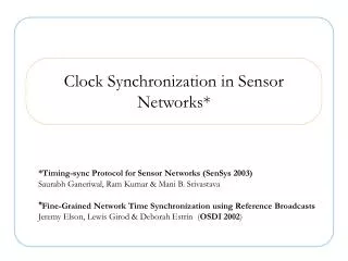
19. Typical Schemes and Algorithms • RBS (Reference Broadcast Synchronization) • TPSN (Timing-Sync Protocol for Sensor Networs) • DTMS (Delay Measurement Time Synchronization) • LTS (Lightweight Time Synchronization) • FTSP (Flooding Time Synchronization Protocol) • TS/MS (Tiny-Sync and Miny-Sync) • TSync • AD (Asynchonous Diffusion)

20. TPSN • Features • Sender-receiver bidirectional mechanism • Two phases of operation: • Level discovery and synchronization • Level discovery phase • Root node initiates level discovery • A node on receiving its level broadcasts it • Any node receiving multiple level packets takes the first one and ignores the others • Any node not receiving a level packet times out and sends a request for level packet

21. Level Discovery Phase 2 1 K B 0 1 A H 1 2 C F 1 2 E L 3 2 2 3 I D G J

22. TPSN • Synchronization phase • Root node sends a start synchronization packet • All nodes of level 1 synchronize themselves to the root node • For every level i, the nodes of that level synchronize to the nodes of level i-1 • If a node in level i-1 is not synchronized, then it does not respond to synchronization requests from level i

23. Time Synchronization Algorithm K B 0 1 A H 1 2 C F 1 2 E L 3 2 2 3 I D G J

24. LTS • Features • Minimize synchronization complexity rather than maximizing accuracy • Authors claim that wireless sensor networks need quite low synchronization accuracy • Sender-receiver bidirectional mechanism • Two LTS algorithms • Centralized • Node sends a synchronization request to a closest reference node by any routing mechanism • Distributed • Requires a spanning tree to be constructed firstly

25. LTS • LTS optimizes synchronization frequency with required precision • The synchronization frequency is calculated from the requested precision, from the depth of the spanning tree, from the drift bound • Simulation results • 500 nodes (120 x 120) • Target precision: 0.5 • Duration: 10 hrs • Centralized: 65% of all nodes request synchronization • 4-5 synchronization operation on average per node • Distributed: • Average 26 pair-wise synchronization per node

26. TS/MS • Features • Determining relative offset and drift between two nodes • Sender-receiver bidirectional scheme • Node 1 sends a probe message to node 2 time-stamped with t0 • Node 2 generates timestamp tb and responds immediately • Node 1 generates timestamp tr • Two clocks c1(t) and c2(t) are linearly related as • C1(t)=a12C2(t)+b12 • The following inequalities are held: • t0<a12tb+b12<tr

27. TS/MS C1(t) = a12H2(t) + b12 C1(t) Sample 3 tr t0 Sample 1 Node 1 Node 2 t0 a12 tb b12 tr tb C2 (t)

28. Parameter Estimation • Relative drift a12 and offset b12 • The tighter the bound, the higher the synchronization precision • Requires high amount of data points and quite complex • Algorithms precision increases with the increased number of data points.

29. Difference Between TS and MS • Different methods in selecting useful data points • Tiny-Sync • Keep only four constrains of all data points • Does nor always give the best solution for the bounds • Mini-Sync is an extension of Tiny-Sync • More optimal solution with increased complexity • Keeps also the data points which may be useful by some future data points to give tighter bounds • A data point is discarded only if it is definitely useless • Quite complex selection criterion.

30. Reference • Elson, Girod, Estrin, “Fine-Grained Network Time Synchronization using Reference Broadcasts” • Sichitiu, Veerarittiphan, “Simple, Accurate Time Synchronization for Wireless Sensor Networks” • Ganeriwal, Kumar, Srivastava, “Timing-Sync Protocol for Sensor Networks” • Genunen, Rabaey, “Lightweight Time Synchronization for Wireless Sensor Networks” • Li, Rus, “Global Clock Synchronization in Sensor Networks” • Dai, Han, “TSync: A Lightweight Bidirectional Time Synchronization Service for Wireless Sensor Networks”

31. Thank you ?