Download
1 / 46
470 likes | 583 Vues
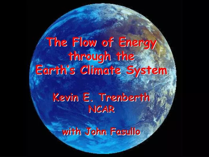
The Flow of Energy through the Earth’s Climate System Kevin E. Trenberth NCAR with John Fasullo. Energy on Earth The main external influence on planet Earth is from radiation.

E N D
The Flow of Energy through the Earth’s Climate System Kevin E. Trenberth NCAR with John Fasullo
Energy on Earth The main external influence on planet Earth is from radiation. Incoming solar shortwave radiation is unevenly distributed owing to the geometry of the Earth-sun system, and the rotation of the Earth. Outgoing longwave radiation is more uniform.
Energy on Earth The incoming radiant energy is transformed into various forms (internal heat, potential energy, latent energy, and kinetic energy) moved around in various ways primarily by the atmosphere and oceans, stored and sequestered in the ocean, land, and ice components of the climate system, and ultimately radiated back to space as infrared radiation. An equilibrium climate mandates a balance between the incoming and outgoing radiation and that the flows of energy are systematic. These drive the weather systems in the atmosphere, currents in the ocean, and fundamentally determine the climate. And they can be perturbed, with climate change.
Energy on Earth Mean and annual cycle of radiation, energy storage and transport are analyzed holistically using datasets: ERBE (Feb 1985 - Apr 1989) 3 satellite configuration; 2 polar orbiting satellites and 1 72-day precessing orbit covering 60N-60S Failure of NOAA-9 (afternoon crossing) in Feb 1987 left only 1 polar orbit (morning) CERES (Mar 2000-present) Terra: single polar orbiting satellite plus Aqua in Jul 2002 NCEP/NCAR Reanalyses ERA-40 Reanalyses JRA-25 Reanalyses World Ocean Atlas ocean data Japanese Meteorological Agency ocean data Global Ocean Data Assimilation System (GODAS)NCEP ECCO: MIT/SCRIPPS/JPL/UH ECCO-GODAE 1992-2004
Fs= .FA - RT+ AE/t • .FO = –Fs – OE/t • Fs = LE + Hs – Rs From ERBE or CERES RT From NRA, ERA-40 or JRA .FA Hs LE Computed as residual Rs LP Fs Ocean heat storage from ocean analyses; transport is zero for global ocean .FO
ERBE was adjusted to have zero net radiation (consistent with ocean obs). Original global adjustment (Trenberth 1997) was modified separately for land and ocean to remove discontinuities exposed in this analysis CERES was similarly adjusted: in OLR to error limits, and albedo to reduce the imbalance of 6.4 W m-2 to an acceptable ~0.9 W m-2 consistent with models and ocean obs.
ERBE Tuning: Inferred Ocean to Land transport of energy The spurious negative trend in implied ocean to land energy transport is addressed in revised tuning. This also has the beneficial effect of yielding a continuous OLR record. Land ERBE revised ERBE from Trenberth 1997 All 12-month running means
Global net flux balance error budget CERES error: Wielicki et al. (2006) W m-2. 1.5
CERES Tuning • Unadjusted, CERES fields depict a net TOA flux of ~6.4 W m-2 which is unrealistic given the reported ocean heat tendency during CERES ~0.4 PW (e.g. Levitus et al. 2005) and model results. • Estimates of the error sources suggest that multiple small error sources combine constructively to yield a bias in the reported imbalance and that both longwave and shortwave budgets require adjustment (Wielicki et al. 2006). • We adjusted OLR +1.5 W m-2 and albedo (+0.3% to 0.30) to give net 0.9 W m-2 consistent with model estimates (e.g. Hansen et al. 2005) and ocean heat uptake (Willis et al. 2004)
Global CERES period March 2000 to May 2004
Net energy flow from ocean to land of 2.2 PW Net imbalance into ocean 0.4 PW CERES period March 2000 to May 2004
Mean annual cycles of albedo and RT Global Note albedo lower in February vs January over oceans (cloud) Global-ocean Global-land shading is ±2 Perihelion Jan 3 Shading represents 2 sampling of monthly means
ASR, OLR, and RT RT= ASR-OLR Global ASR peaks in February, 1 month after perihelion, owing to albedo decrease in February Global-ocean Global-land Main OLR annual cycle from land (snow and temperature) shading represents ±2σ
Annual Cycle of RT (ERBE) ASR OLR NET
Atmospheric total energy divergence (FA) and tendency (AE/t) Global global-ocean global-land Main ocean to land energy transport is in northern hemisphere in northern winter Global =0
Pinatubo SSMI ATOVS Net ocean to land energy transport 12-month running means for ERBE and CERES RT over land and AE/t.
Global, global-ocean, and global-land (from CLM3) estimates of net upwards surface flux (FS) using ocean (red) and land (dotted red).
Amplitude of OE much too large: we can show that the main discrepancies arise from south of 30S where ocean sampling poor. GODAS better than WOA. OE from WOA, GODAS and JMA (shading). FS has been integrated in time to provide OE anomalies
Annual zonal means GODAS > JMA,WOA Departures from annual mean Differences from GODAS exceeding 2 over southern oceans ....WOA>GODAS \\WOA<GODAS
Zonal integral over the world oceans of a) OE’ b) OE/t c) •FO in PW deg-1.
Ocean Transports Comparisons of annual means with direct ocean transect estimates shows good results except slightly lower for Atlantic and global mean
26.5N Atlantic Variability of MOC is large: average overturning is 18.7 ± 5.6 Sv (1 s.d) (range: 4.0 to 34.9 Sv) Cunningham et al 2007 Science
82-83 EN 97-98 EN NRA divergence of energy Total DSE LE 1980 1984 1988 1992 1996 2000
82-83 EN 97-98 EN ERA-40 divergence of energy Total DSE LE 1980 1984 1988 1992 1996 2000
82-83 EN 97-98 EN JRA divergence of energy Total DSE LE 1980 1984 1988 1992 1996 2000
Correlations total energy divergence: Monthly Anomalies JRA vs ERA-40 JRA vs NRA NRA vs ERA-40
SSM/I Pinatubo NOAA-9 to 11 Spurious low frequency variability Deficient low frequency variability on all time scales
0.4 PW into ocean implies 1.26x10²³ J/decade
JRA Reanalyses Large spurious variability associated with satellite transitions • TOVS to ATOVS in Nov 1998 • NOAA-11 to 14 in 1995 • NOAA-9 to 11, late 1988 • SSM/I in July 1987 ERA-40 Reanalyses Large spurious variability associated with Pinatubo and satellite transitions NRA Reanalyses Variability much too low
Ocean analyses Large spurious variability associated with inadequate sampling (esp. southern hemisphere) and changing observations (esp. XBT to ARGO), and uncertainties in XBT drop rates Satellite data Lack of continuity and absolute calibration also gives spurious variability and unreliable trends
Conclusions • We have a new estimate of observed global energy budget and land vs ocean domains • A holistic view of the energy budget allows us to narrow estimates and highlight likely sources of errors. • Low frequency variability in atmosphere and ocean is highly uncertain based on analyses • We need to be able to do a full accounting of the energy storage and flows to determine what is happening to the planet and why the climate is changing. • We can and must do better: but observations from space are in jeopardy, and in situ observations also need improvement • We have used these to evaluate climate and weather models