Download
1 / 56
560 likes | 694 Vues
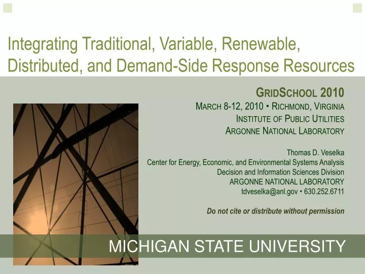
Integrating Traditional, Variable, Renewable, Distributed, and Demand-Side Response Resources. GridSchool 2010 March 8-12, 2010 Richmond, Virginia Institute of Public Utilities Argonne National Laboratory Thomas D. Veselka Center for Energy, Economic, and Environmental Systems Analysis

E N D
Integrating Traditional, Variable, Renewable, Distributed, and Demand-Side Response Resources GridSchool 2010 March 8-12, 2010 Richmond, Virginia Institute of Public Utilities Argonne National Laboratory Thomas D. Veselka Center for Energy, Economic, and Environmental Systems Analysis Decision and Information Sciences Division ARGONNE NATIONAL LABORATORY tdveselka@anl.gov 630.252.6711 Do not cite or distribute without permission MICHIGAN STATE UNIVERSITY
The Grand Challenge of Integrating Renewable Resources with Variable and Intermittent Production into the Grid Is the Ability to Respond to Rapid and Unpredictable Fluctuations Total of 3 Sites Rapid Ramping The thermal system or loads need to adjust quickly Wind Output (MW) Wind is not Always Available when Needed Most Day of the Month in August
Wind Probability Profiles Vary Seasonally and by Time of Day On Average, Wind Output Decreases in the Morning When Load Is Rapidly Increasing. The Opposite Occurs in the Evening. Wind Production (MW) Winter Wind Is Greater Than Summer Wind Summer Nighttime Wind Is Less than Daytime Wind Exceedance Probability (%)
Wind Resources Vary Widely Across the United StatesOften the Best Wind Resources Are Far from Major Load Centers MISO Transmission PJM Transmission 765 kV
The U.S. has Installed the Most Wind Capacity in the World, but the Percent Penetration Rate (% Production) Is Relatively Small U.S. recently became the world leader in wind power with over 8 GW installed in 2008 and 25 GW total installed capacity (AWEA, Feb 09)
U.S. Wind Capacity Growth Source: AWEA 2009
Does Wind Power Influence Market Operations? Wind power ramping events Midwest ISO Wind Power and MN Hub Prices, May 11-17, 2009: http://www.midwestiso.org/ Negative prices (LMPs)
There Are Several Different Types of Photovoltaic Technologies, Each of Which Has its Own Set of Attributes One Size Does Not Fit All Luminescent Solar Concentrators with Multijunction Cells (~40%)
Photovoltaic Efficiencies Have Increased Dramatically Since the Mid-1970’s and Are Expected to Continue Improve Source: http://en.wikipedia.org/wiki/Solar_cell
Public Service Company of Colorado Solar Study200 MW of PV & 200 MW CSP with 800 MWh Storage Source: http://www.xcelenergy.com/SiteCollectionDocuments/docs/PSCo_SolarIntegration_020909.pdf
Spanish PV Study: Annual Hourly Photovoltaic Output Generation (kW) 6 7 8 9 10 11 12 13 14 15 16 17 18 19 20 21 22 Source: http://www.icrepq.com/ICREPQ'09/abstracts/520-ramon-abstract.pdf
Most States Have a Renewable Portfolio Standard (RPS) WA: 15% by 2020* ME: 30% by 2000 New RE: 10% by 2017 VT: (1) RE meets any increase in retail sales by 2012; (2) 20% RE & CHP by 2017 MN: 25% by 2025 (Xcel: 30% by 2020) MT: 15% by 2015 • NH: 23.8% by 2025 ND: 10% by 2015 MI: 10% + 1,100 MW by 2015* • MA: 15% by 2020+1% annual increase(Class I Renewables) • OR: 25% by 2025(large utilities)* 5% - 10% by 2025 (smaller utilities) SD: 10% by 2015 WI: Varies by utility; 10% by 2015 goal • NY: 24% by 2013 RI: 16% by 2020 CT: 23% by 2020 • NV: 25% by 2025* IA: 105 MW • OH: 25% by 2025† • CO: 20% by 2020(IOUs) 10% by 2020 (co-ops & large munis)* • PA: 18% by 2020† • IL: 25% by 2025 VA: 15% by 2025* • NJ: 22.5% by 2021 CA: 20% by 2010 UT: 20% by 2025* KS: 20% by 2020 • MD: 20% by 2022 • MO: 15% by 2021 • AZ: 15% by 2025 • DE: 20% by 2019* • NC: 12.5% by 2021(IOUs) 10% by 2018 (co-ops & munis) • DC: 20% by 2020 • NM: 20% by 2020(IOUs) • 10% by 2020 (co-ops) TX: 5,880 MW by 2015 29 states & DChave an RPS 5 states have goals HI: 40% by 2030 State renewable portfolio standard Minimum solar or customer-sited requirement * State renewable portfolio goal Extra credit for solar or customer-sited renewables † Solar water heating eligible Includes separate tier of non-renewable alternative resources Standards Should be Consistent with Renewable Resources & Needs Source: www.dsireusa.org / September 2009
Currently, Volatility in Production from Variable Resources Are Accommodated by Changing Thermal Unit and Hydroelectric Power Plant Production Levels Operating Capacity The Greater the Operational Flexibility of Dispatchable Units, the more Variability the Grid Will Accommodate Ramp Up Rate Load Following Range Ramp Down Rate Min Output Cold Start Time Minimum Down Time Output (MW) Minimum Up Time Time
Some Technologies Are Able to Come On-line Quickly to Respond to Rapid Load Changes while Others Respond More Slowly Weeks for Shutdown and Startup Some Hydropower Plants Change Very Quickly
The Load Following Range Is Restricted by the Output Minimum and Generation Capacity Operating Capacity Ramp Up Rate Load Following Range Ramp Down Rate Minimum Output Production (MW) Cold Start Time Minimum Down Time Minimum Up Time Time
Highest Production Costs GT NGCC Cycling Coal Lowest Production Costs Nuclear Ideally, Units Are Dispatched Based on Production Cost Max Load Gas Turbines 80 $/MWh NGCC 41 $/MWh Supply (MW) Load (MW) Cycling Coal 32 $/MWh Min Load Base Load Coal Coal 25 $/MWh Nuclear 12 $/MWh Resource Stack 1 2 3 4 5 6 7 8 9 10 11 12 13 14 15 16 17 18 19 20 21 22 23 24 Hour of the Day
Highest Production Costs GT NGCC Cycling Coal Lowest Production Costs Nuclear Unfortunately, a Steam Plant (e.g., Cycling Coal) Does not Have the Flexibility to Operate at a Very Low Output Level Max Load GT Operations Ramp Down Ramp Up Load (MW) Min Load Base Load Coal 1 2 3 4 5 6 7 8 9 10 11 12 13 14 15 16 17 18 19 20 21 22 23 24 Hour of the Day
Wind Generation Wind Production Will Serve Some of the Load.This Production Reduces the Loads that Are Served by other Generating Resources Max Load Ramp Down Ramp Up Load/Wind Output (MW) Min Load 1 2 3 4 5 6 7 8 9 10 11 12 13 14 15 16 17 18 19 20 21 22 23 24 Hour of the Day
New Max Wind Typically Increases Resultant Load Changes New Min Dispatchable Units Serve a Load Profile that Typically, but not Always, Has Greater Fluctuations Relative to the Case where there Is no Wind Ramp Down Larger Range of Operations Ramp Up Load (MW) 1 2 3 4 5 6 7 8 9 10 11 12 13 14 15 16 17 18 19 20 21 22 23 24 Hour of the Day
Highest O&M Costs GT NGCC Coal May Operate Less Efficiently @ Min Gen Cycling Coal Base Load Coal Lowest O&M Costs Nuclear Unit Dispatch with WindResults in Less Thermal Generation & Associated Air Emissions Without Wind Load (MW) With Wind 1 2 3 4 5 6 7 8 9 10 11 12 13 14 15 16 17 18 19 20 21 22 23 24 Hour of the Day
Wind and other Renewable Technologies Will Reduce Greenhouse Gas Emissions 20 Percent Wind by 2030 Report: CO2 Emissions Are Estimated at 25 Percent Lower Than a No-Wind Scenario
As a Result of Variable Resource Generation Some Units Will Operate at a Different Efficiency Point Hydro Combined Cycle Nuclear Diesel Fossil Steam
Highest O&M Costs GT NGCC Cycling Coal Base Load Coal Lowest O&M Costs Nuclear Unit Dispatch with GreaterNighttime Wind Base Load Coal Unit May Need to Be Taken Off-line for Several Hours Without Wind Load (MW) With Wind Sell 1 2 3 4 5 6 7 8 9 10 11 12 13 14 15 16 17 18 19 20 21 22 23 24 Hour of the Day
Upper Reservoir Energy is Produced When Generating Substation Energy is Consumed When Pumping Lower Reservoir Pumped Storage Plants Can Be Used to Help Smooth Out Loads Served by Other Dispatchable Resources React to Sudden Changes in Variable Resource Production Pump Fill Load Valley (Consume) to Utilize Low Cost Production and Avoid Expensive Shutdown Costs Load (MW) Hour of the Day
When a Unit Is Forced Out of Service, the System Responds by Altering the Dispatch 2,500 2,500 Least-Cost Resource Stack Before Outage Least-Cost Resource Stack After Outage 2,250 2,250 • Unprepared • Slow Transition 2,000 2,000 1,750 1,750 Coal Steam Partially Loaded 1,500 1,500 1,200W 80$/MWh 1,200W 40$/MWh Supply - Nuclear Unit Out of Service (MW) Supply Stack without Maintenance (MW) 1,250 1,250 Cycling Coal 40 $/MWh Gas Turbines 80 $/MWh 1,000 1,000 Base Coal 25 $/MWh NGCC 60 $/MWh Operational Problems After the outage it will take hours for the system to reach the least-cost state of operations All demand will not be served 750 750 Cycling Coal 40 $/MWh 500 500 Nuclear 8 $/MWh Base Coal 25 $/MWh 250 250 0 0 Supply Supply Marginal Cost Marginal Cost
Spinning Reserves Help Alleviate Operational Problems Associated with Random Outages 2,500 2,250 2,500 2,000 2,250 1,750 2,000 1,500 1,750 Supply - Nuclear Unit Out of Service (MW) Fast Transition 1,200 MW 80$/MWh 1,200 MW Load 80 $/MWh 1,250 1,500 SimultaneouslyRamp Operations 1,000 Supply Stack without Outages (MW) 1,250 Spinning Reserves NGCC 250 MW NG Steam 110 MW Oil Steam 110 MW Gas Turbines 30 MW Total 500 MW Gas Turbines Gas Turbines 80 $/MWh 750 1,000 NGCC 60 $/MWh NGCC 60 $/MWh Cycling Coal 40 $/MWh 500 750 Cycling Coal 40 $/MWh Base Coal 25 $/MWh 250 500 Base Coal 25 $/MWh Nuclear 8 $/MWh 250 0 Supply 0 Supply Marginal Cost
System Operators Need to Make Certain that Ramping Resources Are Available 2,500 2,500 2,250 2,250 2,500 8 AM Load 1800 MW 7 AM Load 1500 MW 6 AM Load 1200 MW 2,000 2,000 2,250 1,750 1,750 Spinning Reserves 500 MW 2,000 Spinning Reserves 500 MW Spinning Reserves 500 MW 1,500 1,500 Old GT 120 $/MWh 1,750 Old GT 120 $/MWh 1,250 Cycling Coal 40 $/MWh Gas Turbines 1,250 Gas Turbines 1,500 NGCC 60 $/MWh NGCC 60 $/MWh 1,000 1,000 Cycling Coal 40 $/MWh Base Coal 25 $/MWh Supply Stack without Maintenance (MW) 1,250 750 Base Coal 25 $/MWh 750 Gas Turbines 1,000 NGCC 60 $/MWh 500 500 Nuclear 8 $/MWh Cycling Coal 40 $/MWh Nuclear 8 $/MWh 750 250 Base Coal 25 $/MWh 250 500 Nuclear 8 $/MWh 0 Supply 0 Supply 250 0 Supply
Usually, the Grid Can Accommodate Relatively Small Amounts of Wind Generation 2,500 2,500 2,250 2,250 2,500 8 AM Load 1800 MW 7 AM Load 1500 MW 6 AM Load 1200 MW 2,000 2,000 2,250 1,750 1,750 Spinning Reserves 500 MW 2,000 Spinning Reserves 500 MW Spinning Reserves 500 MW 1,500 1,500 Old GT 120 $/MWh 1,750 WIND 1,250 Cycling Coal 40 $/MWh Gas Turbines 1,250 1,500 NGCC 60 $/MWh NGCC 60 $/MWh 1,000 Ramp up due to wind decrease 1,000 Cycling Coal 40 $/MWh Base Coal 25 $/MWh Supply Stack without Maintenance (MW) 1,250 750 Base Coal 25 $/MWh 750 WIND 1,000 NGCC 60 $/MWh 500 500 Nuclear 8 $/MWh Cycling Coal 40 $/MWh Nuclear 8 $/MWh 750 250 Base Coal 25 $/MWh 250 500 Nuclear 8 $/MWh 0 Supply 0 Supply 250 0 Supply
The Unpredictability of Wind Compounds Grid Integration Problems Forecast of Wind Power Production Levels Can Be Made for the Next Few Days Eyeballing: Looks pretty good Mean absolute error is 9.3% But devil is in the details (ramps) Source: Iberdrola Renewables, 2009
Error depends on several factors Prediction horizon Time of the year Terrain complexity Model inputs and model types Spatial smoothing effect Level of predicted power Wind Forecasts Are Far from Perfect in the Short-Term and Much Worse in the Long-Term Error in meteorological forecasts Errors in wind-to-power conversion process Errors in SCADA information and wind farm operation Magnitude Error Phase Error
Source: Smith et al., IEEE Power and Energy Magazine, Vol. 7. No.2, 2009. Technology Improvements Are Alleviating Some Problems Example: The Danish Horns Rev Wind Farm Is Providing Regulation (Frequency Response) and Balancing Response Control Wind Output with Blade Pitch (Spill Energy)
Historical Winter Load Shapes and Wind Generation in the Midwest Unit Commitment Study Wind ~ 14% of Load Source: http://www.dis.anl.gov/pubs/65610.pdf
Problem: Given that Wind Forecasts Have Errors, Make an Economic Unit-Commitment Schedule that Is Reliable Costs: Generation, Unserved Energy, & Startup Constraint: Ramping, Up & Down Time, Min Output, & Maintain Reserves Wind can be curtailed (spilled energy) Source: http://www.dis.anl.gov/pubs/65610.pdf
Unit Commitment Results Using Various Modeling Methodologies and Assumptions Stochastic UC gives higher commitment & more available operating reserves Similar result for deterministic UC w/additional reserve requirement Source: http://www.dis.anl.gov/pubs/65610.pdf
Comparison of Costs (30 day simulation)Results Based on Fixed Unit Commitments and Real-Time Economic Dispatch • The potential value of forecasting illustrated by perfect forecast (D1) • Deterministic UC with point forecast (D2) appears too risky • Deterministic UC w/add reserves (D3) and stochastic UC (S1) give similar total cost Source: http://www.dis.anl.gov/pubs/65610.pdf
Finding the “Best” Mix of Generating Capacity to Backup Variable Resources While Keeping Costs Reasonable Is Challenging * Operating costs includes fuel costs and fixed and variable operating and maintenance costs ** Operating flexibility is the unit’s ability to respond to load changes and includes ramp rates, cold start time, etc. Zero Fuel Costs • Desirability Rating • Very Low • Moderately Low • Average • Moderately High • Very High Variability Issues
Suggested Reading: DOE’s 20% Wind by 2030 Report • Explores “a modeled energy scenario in which wind provides 20% of U.S. electricity by 2030” • Describes opportunities and challenges in several areas • Turbine technology • Manufacturing, materials, and jobs • Transmission and integration • Siting and environmental effects • Markets • Enhanced wind forecasting and better integration into system operation is one of the challenges • DOE is funding several research projects in this area
Thank you for your attention Source: BOR
Reserve Capacity Is Needed to Serve Load when One or More Generators Are Out of Service MW Total System Capacity Upper RM Peak Load Forecast Lower RM New Capacity Additions Existing System Capacity Engineering Guideline Build 15% to 20% more capacity than the peak load Years
Variable Resources Have a Capacity Value Which Can Be Approximated Using Probabilistic Methodologies Probability of 3 sixes = 1/6 x 1/6 x 1/6 = 1/216 = less than %0.5
Max Load Min Load Loads Can Also Be Viewed as Probabilistic Events Step 1: Chronological Loads Load (MW) 1 2 3 4 5 6 7 8 9 10 11 12 13 14 15 16 17 18 19 20 21 22 23 24 Hour of the Day
Load Time Min Load Sorted Summer Load ProfileStep 2: Load Exceedance Curve Max Load hr 17 Some Information Is Lost Such as Load Changes Over Time hr 17 hr 4 Load (MW) hr 4 0 100 Exceedance Probability (%)
Max Load Is Never Exceeded GT NGCC Load Time Cycling Coal Min Load Is Always Exceeded Unit Production Levels Can Be Estimated Using a Load Duration Curve Information Such as Unit Ramping and Frequency of Unit Starts/Stops Are Lost Load (MW) Base Load Coal Nuclear 0 100 Exceedance Probability (%)
GT Load NGCC Time Cycling Coal When a Supply Resource Is Forced Out of Service Other Resources Are Dispatched to Serve the Load Max Load Load (MW) Min Load Base Load Coal Nuclear Forced Out of Service 1 2 3 4 5 6 7 8 9 10 11 12 13 14 15 16 17 18 19 20 21 22 23 24 Hour of the Day
New Max Load not Served by the Nuclear Unit Is Satisfied by Other Units in the Resource Stack Load GT Time New Min NGCC Nuclear Capacity Cycling Coal Base Load Coal Nuclear Alternatively, the Load Curve Can Be Adjusted While Including the Out-of-service Unit Load (MW) Original Curve 1 2 3 4 5 6 7 8 9 10 11 12 13 14 15 16 17 18 19 20 21 22 23 24 Hour of the Day
New Max Nuclear Capacity GT NGCC Cycling Coal New Min Base Load Coal Nuclear The Same Methodology Can Be Applied to a Load Duration Curve Load (MW) Original Curve Exceedance Probability (%) 0 100
Area = Outage Rate/100 X Nuclear Capacity GT Weighted Average Curve of NuclearUnit On & Off NGCC Cycling Coal Equivalent Load Curve Accounts for Nuclear Outages Base Load Coal There Is Some Probability that a Unit Does Not Operate Nuclear Capacity Nuclear Off We don’t know with certainty if the nuclear unit will be either on or off at some point in the future Nuclear On Load (MW) Nuclear 0 100 Exceedance Probability (%)