Download
1 / 28
280 likes | 465 Vues
Using Pseudo RAOB Observations to Study GFS Skill Score Dropouts . NOAA/NWS/NCEP/ Environmental Modeling Center Jordan C. Alpert, Brad Ballish, Da Na Carlis, V. Krishna Kumar. 5A.6 AMS 23WAF_19NWP Conf, 1-5 June 2009, Omaha, NE.

E N D
Using Pseudo RAOB Observations to Study GFS Skill Score Dropouts NOAA/NWS/NCEP/ Environmental Modeling Center Jordan C. Alpert, Brad Ballish, Da Na Carlis, V. Krishna Kumar 5A.6 AMS 23WAF_19NWP Conf, 1-5 June 2009, Omaha, NE
Using Pseudo RAOB Observations to Study GFS Skill Score Dropouts NOAA/NWS/NCEP/ Environmental Modeling Center Jordan C. Alpert, Brad Ballish, Da Na Carlis, V. Krishna Kumar The “Dropout” Team 5A.6 AMS 23WAF_19NWP Conf, 1-5 June 2009, Omaha, NE
Need to find a Remedy for the Dropouts Determine if “dropouts” are from QC, GSI analysis, GFS forecast model • Define Dropout (verification web page stats) • Quantify Dropout Events • If QC is responsible then construct (implement) a real time monitoring (detection/correction) system. • Determine Common Threads in Dropout Cases
What is a “dropout”? The criteria that a 5-day 500 mb Anomaly Correlation (AC) height score must meet in order to be considered a dropout (Alpert et al, 2009) : • At least one of the following criteria must be met: • a) ECMWF minus GFS ≥ 15 AC points • b) GFS AC ≤ 0.70 • c) ECMWF AC ≤ 0.75 • d) Monthly avg GFS AC score minus GFS forecast ≥ 15 • e) Monthly avg ECMWF AC score minus ECMWF forecast ≥ 15 • Criteria is for NH and SH dropouts. On approximately a monthly basis, poor forecasts or “Skill Score Dropouts” plague GFS performance. GFS production in Black, ECMWF in Red.
Tools to compare ECMWF and NCEP Dropouts • Use ECMWF analysis to generate “Pseudo Obs” for input to the Gridded Statistical Interpolation (GSI) and GFS forecasts. • Generate a Climatology of NH and SH dropouts – what are the systematic differences • Interpolate ECM and GSI analyses to observations to determine comparative strengths and weaknesses. • Statistically analyze observation type fits • stratify by pressure, type, and difference magnitude Goal: Diagnose Quality Control problems to implement real-time QC detection/correction and improvements to analysis system algorithms
Poor Forecasts or Skill Score “Dropouts” Lower GFS Performance. For this Dropout see IC on next slide...
Trough in central Pacific shows differences between ECMWF (no dropout) and GFS (had dropout) Ovrly “patch” box ECM in this area but GSI elsewhere
Oct. 22,2007 Pacific OVRLY F00 GFS: NCEP Ops ECMWF: ECMWF Ops ECM: ECMWFGSI OVRLY: Patch
F120 GFS: NCEP Ops ECMWF: ECMWF Ops ECM: ECMWFGSI OVRLY: Patch
ECMWF INITIAL CONDITIONS FOR GFS FORECASTS “ECM” Runs” ECM(WF) Analysis 1x1 deg, 14 levels ------------------------- PSEUDO ECM RAOBS ( ) INPUT ----------- OUTPUT
ECMWF INITIAL CONDITIONS FOR GFS FORECASTS “ECM” Runs” ECM(WF) Analysis 1x1 deg, 15 levels ------------------------- PSEUDO ECM RAOBS PSEUDO ECM RAOBS GFS GUESS -------------- ECM ANLYSIS “PRE-COND” GUESS ( ) INPUT ----------- OUTPUT
ECMWF INITIAL CONDITIONS FOR GFS FORECASTS “ECM” Runs” ECM(WF) Analysis 1x1 deg, 15 levels ------------------------- PSEUDO ECM RAOBS PSEUDO ECM RAOBS GFS GUESS -------------- ECM ANLYSIS “PRE-COND” GUESS Run GSI ----------- Analysis PRE-COND ECM GUESS PSEUDO ECM RAOBS --------------- ECM ANL ( ) INPUT ----------- OUTPUT
ECMWF INITIAL CONDITIONS FOR GFS FORECASTS “ECM” Runs” ECM(WF) Analysis 1x1 deg, 15 levels ------------------------- PSEUDO ECM RAOBS PSEUDO ECM RAOBS GFS GUESS -------------- ECM ANLYSIS “PRE-COND” GUESS Run GSI ----------- Analysis PRE-COND ECM GUESS PSEUDO ECM RAOBS --------------- ECM ANL ( ) INPUT ----------- OUTPUT Run GSI again
ECMWF INITIAL CONDITIONS FOR GFS FORECASTS “ECM” Runs” ECM(WF) Analysis 1x1 deg, 15 levels ------------------------- PSEUDO ECM RAOBS ECM ANL ------------ GFS 5-d FORECAST PSEUDO ECM RAOBS GFS GUESS -------------- ECM ANLYSIS “PRE-COND” GUESS Run GSI ------------ Analysis PRE-COND ECM GUESS PSEUDO ECM “OBS” --------------- ECM ANL ( ) INPUT ----------- OUTPUT Run GSI again
ECMWF INITIAL CONDITIONS FOR GFS FORECASTS “ECMCYC” Runs” PSEUDO ECM “OBS” Production GFS GUESS ------RUN GSI------ ECM ANLYSIS 00Z First Time Make 3,6,9-h GFS forecast 00Z Pseudo OBS 3,6,9-h GUESS ----RUN GSI---- ECM ANALYSIS Make 3,6,9-h GFS forecast Make 3,6,9-h GFS forecast ( ) 18Z Pseudo OBS 3,6,9-h GUESS ----RUN GSI---- ECM ANALYSIS INPUT ----------- OUTPUT Make 3,6,9-h GFS forecast Figure 2. Schematic representation of an ECM run using the GSI/GFS system and ECMWF 14 level pressure and 1x1 degree analysis files.
ECMCYC ECMCYC
5 Day Anomaly Correlation Scores at 500 hPa for Dropout Cases ECM Performs Better than GFS (NH) 2007-2008 • ECM runs (blue) are a good representation for ECMWF analysis • OVRLY runs (green) with ECM psuedo-obs over the Central Pacific drastically improve two October 2007 dropout cases (102200 & 102212).
ECM runs (blue) in the SH do almost as well as ECMWF CNTRL runs (green) improve upon GFS scores 9 of 10 times but only alleviates about half of the dropouts, but large skill gap remains.
Figure 10. Impact of satellite radiance data on Southern Hemisphere dropouts. 5-day anomaly correlation scores shown for 10 cases. MINDATA is the GFS/GSI run with only TRMM and SSMI data present, PREPB is the GFS/GSI run with only conventional observations (i.e. RAOB, satellite winds, profiler, etc..), AMSUA is the GFS/GSI run with conventional observations and amsua satellite radiance data, AMSUB is the GFS/GSI run with conventional observations and amsub satellite radiance data, MHS is the GFS/GSI run with conventional observations and mhs satellite radiance data, GPSRO is the GFS/GSI run with conventional observations and gpsro satellite radiance data, AIRS is the GFS/GSI run with conventional observations and airs satellite radiance data, HIRS is the GFS/GSI run with conventional observations and hirs satellite radiance data, and CNTRL is the GFS/GSI run with conventional observations and all satellite radiance data present with a 6-hr data ingest window.
Figure 11. Impact of satellite radiance data on Southern Hemisphere dropouts. 5-day root-mean-error scores shown for 10 cases. The experiments are named the same as Fig. 10.
Impact of Conventional and Satellite Radiance Obs on 3-d and 5-d GFS Forecasts • Satellite radiance data shows positive impact on NH 3-D and 5-D forecasts • In the SH, conventional (PREPB alone) show a large negative impact (8 points) in 5-D forecasts! -- another puzzle • Addition of satellite radiance data to conventional and satellite observations have a positive impact on 5-D forecasts • AMSUA along with PREPB conventional observations (yellow) show the largest positive impact in the NH and SH experiments and typically are correlated with the results of the CNTRL • This is confirmed by other studies (ECMWF and Joint Center) and shows how each case has individual characteristics requiring incisive diagnostics.
Summary • ECM analyses show dropouts can be alleviated in GFS forecasts • Running the operational GSI with an ECM derived background guess results in better forecast skill than the operational GFS but not as good as ECM runs • Running the GSI after removing selected observation types offers a systematic approach for assessing the impact of different observation types • Quality control problem detection and correction algorithms per observation type maybe be possible using analysis differences and areas of potential activity like baroclinic instability index
Future Work • ECM analyses show dropouts can be alleviated in GFS forecasts • Expand Dropout Team • Additional effort focused on improving GFS QC and Model • Augmented and corrected observation data base information (Ballish, et al 2009) • Develop and test bias correction for conventional observations • Diagnose potentially important impact of humidity through satellite data and improve use of current satellite data • Negative moisture in background model field - Continue to develop global model • Test Sat wind QC e.g., Develop and test thinning (a Super-Ob strategy) • Develop use of ODB for diagnostics and verification • Construct a detection system of Dropouts (Cycle ECM runs to compare with production) • Battery of Diagnostic displays for examination based on an alarm or event • Detection and event recognition to trigger alarms to start offline procedures for post mortem • Explore additional diagnostic tools • Adjoint techniques • Obs. Sensitivity • Bishop & Toth (THORPEX WSR Targeting Technique) • Kalnay (EnKF Technique)
SH Dropout Composite Cntrl vs InterpGES SH CNTRL 5-day Composite AC = 0.71 SH InterpGES 5-day Composite AC = 0.73 Zonal average (above) and mean composite difference between GFS Cntrl and InterpGES (Increments). GFS has low level SH warm “bias” if we consider ECMWF as ground truth.
c) Figure 3. The total Eady Baroclinic Index (EBI) (day -1) at 500 hPa for the F00 forecast from the August 16, 2008, 00 UTC (2008081600) initial conditions for the a) GFS model, and b) ECM model with two iterations of the GSI and from April 13, 2009 12 UTC for the ECMCYC run. Note the difference in the dates.
AMSUA GPSRO 18% loss 36% loss MHS HIRS4 32% loss 33% loss AIRS QSCAT 100% loss 100% loss Figure 13. Satellite data counts for the period 20081230-20090107 covering the 5-day forecast dropout initializing on 2009010312.